Paper · adjacent
Full-bandwidth Transformer
arXiv:2608.08888 · PDF · code
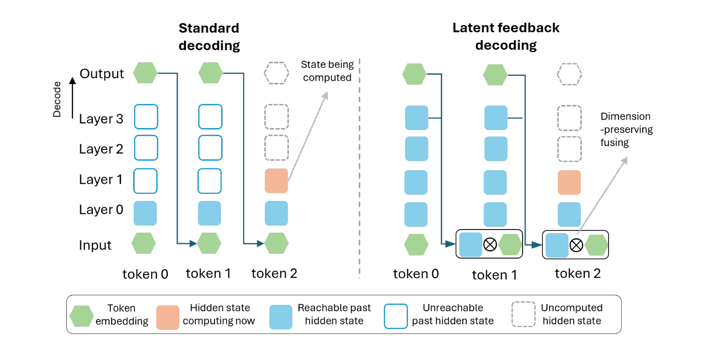
Feeding the previous decoding step's top-layer hidden state back into the next input, fused with the sampled token's embedding, lets every layer read the past as the whole stack processed it, for two matrix multiplications per token and no change to the architecture or the KV cache. A few parallel passes late in pretraining are enough to train it, and 1B-parameter models trained this way match or approach standard models trained on roughly 1.5 times the tokens and, before instruction tuning, often reason in fewer tokens.
AI-drafted summary, not yet reviewed by a person. Written from: full text (arXiv v2), appendices included; the lead author's thread, posted with the first version; the lead author's thread on the revision; the senior author's post quoting the first thread, and his thread on where the idea came from.
The paper in brief
- Problem. “Dense attention gives each token broad horizontal access to the past, but the vertical feedback channel between decoding steps remains narrow: only the sampled token returns to the bottom of the stack, while the top-layer hidden state is discarded.” (Abstract.)
- Why it matters. What a model computes and does not put into a token stays at the layer that computed it: it “is not erased, intermediate activations persist in the KV cache, but it is depth-frozen”. So “Verbalization is thus the only channel for information to re-enter the bottom layer and receive fresh computation, at the cost of being squeezed through a single token, forcing the model either to spend tokens narrating its intermediate state or recompute that state from scratch at every position.” (§1.)
- Question. The introduction states a proposal and no question: “we propose the full-bandwidth transformer where we widen this channel to its full width” (§1). The question the authors say they began from is in the discussion that closes the paper: “This led us to ask whether a transformer could be trained recursively in parallel by feeding back soft latent belief states across multiple passes.” (After §7.)
- Answer. “With negligible per-token decoding overhead, full-bandwidth transformers match or approach standard transformers trained with roughly 1.5× more tokens, and manage to produce shorter reasoning when no off-policy templates are provided.” (Abstract.)
The three claims are a chain. The first is the mechanism and what it costs to run. The second is what makes it trainable, since a model that has never had a hidden state in its input cannot use one. The third is what the trained models do.
- Feeding the previous step’s top-layer hidden state back into the next input, fused with the sampled token’s embedding, lets every layer read the past as the whole stack processed it, for two matrix multiplications per token and no change to the architecture, the KV cache or the training objective.
- The feedback can be trained without giving up parallel training over positions: a few parallel passes stand in for the recurrence, they are needed only late in pretraining, and a small share of deeper passes keeps the feedback stable far past the depth it was trained at.
- A 1B-parameter model trained this way matches or approaches standard models trained on more tokens, and before instruction tuning it often reasons in fewer tokens.
What the paper starts from
Terms.
- Horizontal and vertical: the two directions a transformer computes in, “the horizontal axis (across positions)” and “the vertical axis (across depth)” (§2).
- Bandwidth: how much of the model’s state a path carries. Across positions, “dense attention is effectively full-bandwidth” (§2). From one decoding step to the next the path is one token: “Decoding compresses the model’s entire top-layer state, a D-dimensional vector, down to a single symbol” (§1).
- Depth-frozen: “a state produced at layer ℓ is readable only by layers above ℓ, so it can never return to the bottom of the stack for further processing” (§1).
- Latent feedback decoding: decoding that “fuses the previous top-layer hidden state with the sampled token’s embedding during decoding, and feeds the result back as the next input” (§1).
- Full-bandwidth transformer: “a transformer capable of decoding this way” (§1).
- The fusion (§3.1, equation 4): a gated linear unit. The previous hidden state is multiplied by a matrix W_H, and each dimension of the result is scaled by a sigmoid of the token embedding multiplied by a second matrix W_G. Both matrices are D by D.
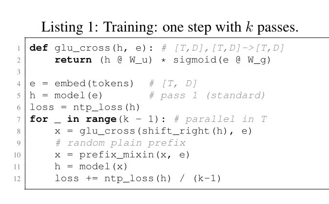
- Feedback pass (§3.2): one more run of the whole stack over a sequence, in parallel across positions, in which each position’s input is its token embedding fused with the top-layer state the previous run produced one position to the left.
- STANDARD, SOFT and FUSED (§4.2): three ways to run a trained model. STANDARD uses token embeddings only: “This evaluates the full-bandwidth model as an ordinary transformer, and measures the cost of latent-feedback training when the feedback channel is not used at inference.” SOFT prefills the prompt once and then decodes with latent feedback. FUSED gives the prompt one more prefill pass, a fused one, and then decodes as SOFT does.
The inference it rests on (§2). A layer of a standard transformer cannot read what deeper layers made of earlier positions, “even though the deeper, more fully processed states of those same positions have already been computed and sit in the KV cache”. That restriction has a use in training: “this depth-wise dependency constraint is also what lets transformers train in parallel across positions”. It has none in generation: “At decoding time, however, generation is already sequential over tokens, so the constraint buys nothing”. The paper takes this as “opening the door to richer dependencies on past hidden states”, and the introduction names what stands in the way: “The obstacle is training.” (§1.)
The setting (§4, Appendix A). Every model is a decoder-only transformer of 1B parameters that the authors pretrain themselves: 24 layers, a hidden state of 1,536 dimensions, a vocabulary of 100,352 tokens with the embedding and the output head tied, and a context of 8,192 tokens. Most layers attend over a sliding window of 2,048 tokens, “while every sixth layer uses full attention”. The training data is “the data mixture of Phi-4”. Each full-bandwidth run is set against standard transformers trained on the same data, at the same number of tokens and at 1T tokens (Figure 5). The runs differ in their schedule, the share of training batches run with one, two or three passes, and so in their token-equivalent compute, “defined as training tokens multiplied by the average number of forward passes per batch”. The last column of the table is that compute (Table 1).
| Run | Schedule | Compute |
|---|---|---|
| 10B | 100% three-pass | 30B |
| 100B | 75% one-pass, 25% three-pass | 150B |
| 200B | 75% one-pass, 22% two-pass, 3% three-pass | 256B |
| 400B (1.28×) | 75% one-pass, 22% two-pass, 3% three-pass | 512B |
| 400B (1.5×) | 75% one-pass, 25% three-pass | 600B |
The measures (§4.1, §4.2). Validation loss. Average accuracy with five in-context examples on ten multiple-choice tasks, which the paper calls 5-shot LM Eval: “RTE, TruthfulQA-MC2, ARC-Easy, ARC-Challenge, BoolQ, PIQA, WinoGrande, OpenBookQA, COPA, and MMLU”. For free-form generation, Pass@1 on GSM8K and MATH-500 and Pass@3 on HumanEval and MBPP, the last “estimated from 10 rollouts per problem, with temperature grid-searched over {0.3, 0.5, 0.7} separately for each decoding regime”. And the median length of a rollout, in tokens.
Tools taken from earlier work. Training a recurrence with parallel passes, which the paper calls temporal parallelism, “following a common strategy for parallelizing recurrent computation during training” (Zeng et al., 2025; Cai et al., 2026; Huang et al., 2026; Liu & Liu, 2026; Danieli et al., 2025). A next-token loss on the output of every pass, as in loop transformers (Zhu et al., 2025; Sharma & Vu, 2026; Shomali et al., 2026). Depth scaling (Yang et al., 2024; Noci et al., 2022). The NorMuon optimizer (Li et al., 2026), a WSD learning-rate schedule (Hägele et al., 2024; Hu et al., 2024), a z-loss (Chowdhery et al., 2023) and AdamC (Defazio, 2025). For serving under vLLM, the buffer used by implementations of EAGLE (Li et al., 2024a) and of multi-token prediction (Gloeckle et al., 2024).
The argument, claim by claim
Claim 1: the top-layer state can be fed back at every step for almost nothing
Feeding the previous step’s top-layer hidden state back with the sampled token lets every layer of the next step read the past as the whole stack processed it. It adds two matrix multiplications per token and changes nothing else in the model or in how it is served.
Evidence. First the design (§3.1). At each step the input to the stack is the fusion of the sampled token’s embedding with the top-layer state of the step before. The paper states what follows from the wiring as two equations. In a standard transformer the states that a position can reach at a given layer are those of earlier positions at lower layers (equation 2). With latent feedback they are those of earlier positions at every layer (equation 5): “Now every layer, including the lowest, can access top-layer information”. The second thing the wiring gives is room to work without writing: “Latent feedback also provides a continuous scratchpad, relieving the pressure to verbalize intermediate state.”
![A listing of code titled 'Listing 2: Inference (SOFT); uncommenting line 2-3 gives FUSED; line 7 shows the STANDARD-decoding input)'. Line 1 prefills: h = model(embed(prompt)). Lines 2 and 3, commented out, run the model again on glu_cross(shift_right(h), embed(prompt)). Lines 4 and 5 sample a token from lm_head(h[-1]) and keep h[-1] as h_prev. The decoding loop, lines 6 to 10: x = glu_cross(h_prev, embed(tok)); a comment, 'standard decoding: x = embed(tok)'; h_prev = model_step(x, kv_cache); tok = sample(lm_head(h_prev)).](/figures/wang2026-full-bandwidth-transformer/fig2-inference.png)
Sketch from Claude
The fusion of equation 4, in 8 dimensions
Every number here is made up, in 8 dimensions where the model has 1,536 (Appendix A). Nothing in it is a result.
The input is the projected state, with each dimension turned down by the gate the token sets. Change the token and the same state is weighted another way. Change the state and the same token feeds a different input.
| dimension | ||||||||
|---|---|---|---|---|---|---|---|---|
| htop-layer state of the step before | 0.80 | 0.10 | 0.60 | −0.50 | −0.30 | 0.70 | −0.60 | 0.40 |
| WH hthe state, projected | 0.82 | 0.26 | 0.34 | −0.42 | −0.19 | 0.39 | −0.48 | 0.43 |
| eembedding of the sampled token | 0.90 | −0.30 | 0.50 | −0.70 | 0.20 | 0.60 | −0.50 | 0.30 |
| σ(WG e)the gate: a multiplier for each dimension, from 0 to 1 | 0.87 | 0.30 | 0.73 | 0.10 | 0.57 | 0.75 | 0.70 | 0.52 |
| xinput fed to the stack: WH h times the gate | 0.71 | 0.08 | 0.25 | −0.04 | −0.11 | 0.29 | −0.33 | 0.22 |
the state the token what the stack is fed what standard decoding would feed
Dimension 1: 0.82 × 0.87 = 0.71. Standard decoding would feed 0.90.
To try. Join them not at all, and switch states. Go back to the gated product, and switch tokens, then states. Scale WH to zero under the gated product, then under addition. Do the same with WG.
Then the cost. The state fed back is one the model has computed anyway, to choose the token. “The added inference cost is independent of context length and model depth.” The extra work is the two matrix multiplications of the fusion, “negligible against a forward pass through L blocks (< 1%)” (§3.1). Measured end to end under vLLM, on one H100 at batch size 1, SOFT decoding runs at 209.1 tokens per second against 214.1 for STANDARD, a slowdown of 2.3% (Appendix L, Table 6).
Then a check that the state arrives where the design says (§4.4, Appendix M, Figure 15). On synthetic sequences whose label is fixed by tokens near the start, a linear probe is fitted at every depth of the last token’s residual stream. With the last token entering as a plain embedding, “the layer-0 probe is near chance”. With the preceding token’s top-layer state fused into it, “layer-0 probe accuracy rises to 99.6% for completion tracking and 100% for delayed memory”. The tasks and the probes are set out in Appendix N.
- Objections it expects.
- That the model will learn to ignore the state. This is the stated reason for the form of the fusion: “The asymmetry is deliberate: the hidden state occupies the value pathway, while the token embedding enters only as a multiplicative gate.” The authors hypothesize that a symmetric fusion “would leave a shortcut open where the model could ignore the h and recover the plain token input” (§3.1). Their own small test does not bear the worry out. With plain addition, and with concatenation and projection, on a 20-layer Nanochat model, “we do not see one method outperform another one on a small scale, nor do we observe that symmetric fusion shows signs of shortcut seeking” (O.1, Figure 20). Wang’s thread on the revision draws the consequence: “So the glu cross gate used in the original version may not be the workable solution.” (post 4.)
- That the gate squeezes the state back down. The learned W_H has numerical rank 1,530 of 1,536, and the gate’s activations “span a broad range between zero and one and vary substantially across tokens” (Appendix O, Figure 17). The authors’ reading: “the fusion gate preserves a high-dimensional channel from the previous hidden state while allowing the current token to selectively reweight it”.
- That it does not fit a serving stack. “The scheme is also vLLM-compatible” (§3.1): the top-layer state of each request is kept in a buffer and copied in before the next step (Appendix B).
- That a probe finding the state is not the model using it. The paper says so itself: “improved decodability does not by itself imply improved output”, and “making state available and causally exploiting it are distinct, and only the downstream task results (Sec. 4) speak to the latter” (Appendix M).
- How far it goes. The paper names two things the feedback is not (§3.1). It is not a register that is overwritten: “Latent feedback is recurrent in form, but past states persist in the KV cache rather than being overwritten, so every earlier state remains readable by the current token.” And it adds no depth: “Latent feedback does not change the asymptotic serial depth of decoding”. “What changes is the bandwidth of the path, with a verbal channel and a continuous channel now evolving in parallel.”
- How strongly it is made. The cost is stated flatly, under a heading that reads “Latent feedback is free to serve.” The benefit is stated as what the wiring allows and what it predicts: the scratchpad “predicts the possibility of shorter rollouts”, for which a later section “provides preliminary evidence” (§3.1). Wang’s first post is stronger about what that buys: “it boosts performance for free” (post 1).
- What it hands on. A model that cannot yet use what it would be fed: “A pretrained model has never seen hidden states in its input, so latent feedback cannot simply be switched on at inference” (§1).
Claim 2: the feedback can be trained in parallel, with a few passes late in pretraining
Training on the recurrence as it runs at decoding would have to go position by position. The paper replaces it with a small number of passes, each parallel across positions, run only in the last quarter of pretraining, and finds that a small share of three-pass batches keeps the feedback stable far past three steps.
Evidence. First the scheme (§3.2). The recurrence of decoding is sequential over positions, so “training on it directly requires RNN-style backpropagation through time (BPTT), which breaks the parallel teacher forcing”. In its place the top-layer states are computed several times. The first pass is an ordinary forward pass. Then “each subsequent pass shifts the previous pass’s states one position rightward, fuses them with the token embeddings, and re-runs the full stack in parallel across all positions”. The next-token loss is applied to the output of every pass, and the loss of the later passes is given a weight of one, set “without any tuning”. Gradients flow back through the passes: “We do not detach the gradient, so the loss from later passes backpropagates into earlier passes’ latent states, acting as an auxiliary objective; this does increase the memory footprint.” With k passes the feedback is trained over k − 1 steps of tokens, and “Training thus pays sequentiality across passes rather than across positions.”
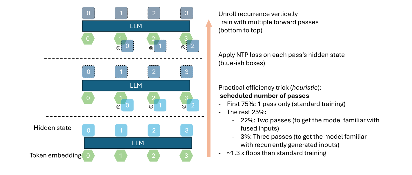
Then the schedule, which is where the cost is kept down. Passes are added late: “This lets the run begin from an ordinary mid-trained checkpoint, spend the bulk of its compute on standard teacher forcing, and pay the extra feedback-pass cost only in the end.” A training iteration takes 0.36 seconds with one pass, 0.75 with two, 1.13 with three and 1.53 with four: “Each additional pass adds approximately 0.4 seconds extra per iteration.” (Appendix D.) Under the schedule of the 200B run, the token-equivalent compute is 256B (Table 1).
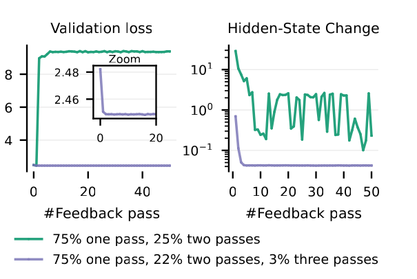
Then the finding about what goes into the schedule (§3.2, Figure 4). The introduction says of it that “the schedule’s composition matters in an unexpected way” (§1). At decoding the feedback is applied once for every generated token, far more times than any number of passes in training: “the trained map must remain stable under many more self-compositions than any training budget can simulate”. Two 1B models are trained on 200B tokens. Trained on one-pass and two-pass batches only, the model does well at two passes and breaks down when more are run. With 3% of batches at three passes, “validation loss remains flat through 30 feedback steps, and the hidden-state change decays to a small plateau”. In the introduction’s words, “mixing in as little as 3% three-pass batches turns the learned map into a stable attractor” (§1). The stability is said to reach decoding: “hundred-token rollouts show no sign of breakdown, and we observe similar stability under k = 1000 feedback passes” (§3.2; the plot is the third panel of the figure in Appendix E).
Two additions close gaps between training and use (§3.2). The first is the prefix mixin. At inference the prompt is plain embeddings and the generated tokens are fused inputs, so in each pass after the first a prefix of random length is put back to plain embeddings, and “Training thus covers sequences that switch from plain to fused inputs at an arbitrary point”. The second is a set of three measures for long runs of feedback. The scale of the top-layer state is kept bounded, by depth scaling and by an RMSNorm on the fused input. The embedding and the readout share their weights, so that the two kinds of input “remain in a compatible basis”. And during training a small uniform noise, with σ = 0.02 in every experiment (§4), is added to the state before fusion. The full code with these included is Figure 10, in Appendix C.
The passes are used twice more once training is over (§5), for two things that a model with a recurrence in it could otherwise only do one token at a time.
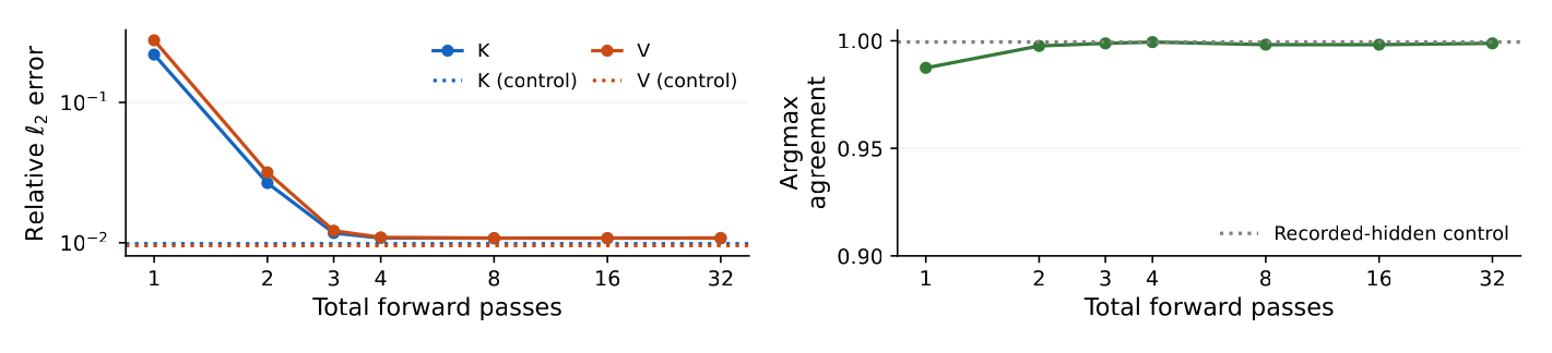
The first is rebuilding a KV cache from stored tokens, “for example when resuming an old request” (§5.1). For tokens generated under SOFT, “ordinary prefill with embeddings as input does not reproduce the original cache”, and replaying the recurrence “requires one dependent forward step per generated token”. Instead the stored tokens are run through several parallel passes and the last pass’s cache is kept. On four greedy MATH-500 rollouts averaging 420 tokens, three passes give a relative error of 1.17% for keys and 1.22% for values, with 99.88% agreement on the next token, and four passes give 1.08% and 1.09%. A single parallel pass given the hidden states actually recorded during decoding still shows 0.99% and 0.95%, so “three to four passes recover the cache close to the numerical discrepancy between parallel and incremental execution on these trajectories” (Figure 8).
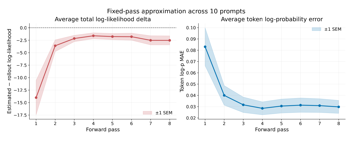
The second is scoring a rollout that another policy sampled, which post-training needs (§5.2). Under latent feedback the likelihood of such a rollout “cannot be evaluated by standard parallel teacher forcing”. Two recipes are set out. One reuses the hidden states of the policy that sampled the rollout, which “introduces bias whenever the latent trajectories of the behavior and policy models differ”. The other approximates the likelihood with a fixed number of parallel passes. On ten prompts, “The approximation error reduces significantly after two forward passes and plateaus after three passes.” (Figure 9.) The paper marks the whole part as untested: “Note that the solutions discussed are hypothetical only and unverified by experiments.” Wang’s thread on the revision reports a first run, which the paper does not have: “Some simple online RL, w/ vLLM as rollout engine, verifies that the full-bandwidth transformer is post-trainable and improvement remains!” (post 5.)
- Objections it expects.
- That the stable schedule is a lucky one. The paper concedes it: “the design of scheduling is mainly based on empirical experiments and failure of convergence does occur when pursuing extreme efficiency” (§3.2). The schedule that is stable at 200B tokens “failed to extrapolate at 400B tokens scale”, and “changing the last stage from three to four passes or having three passes across the last 25% fixes the instability” (Appendix E).
- That the passes could be spread through training, and fewer of them used. Interleaving one-pass and multi-pass steps “prevents continuing from a mid-train checkpoint and shows suboptimal performance compared with having each stage in bulk” (§4.4, Appendix O, Figure 16).
- That gradients need not flow between passes. Trained with the states detached, the models “still show improved validation loss in second pass, however their level of improvement is much smaller compared with the non-detached version” (Appendix O, Figure 16).
- That the stability measures are doing the work. One of the three was tested. The noise “slightly improves the loss, especially under standard prefilling”, and “is not observed to change the stable attractor pattern” (Appendix O, Figure 19). Of the other two: “we did not ablate the depth scaling and weight tying” (§3.2).
- How strongly it is made. As a recipe found by trial. “Current feedback pass scheduling is based on a heuristic” (§7). “The exact reason for converging in 3 passes is also unclear” (§3.2). Of the stability measures: “We adopted these techniques in that we hypothesize that they are, motivationally, the right thing to do, which may not be actually necessary empirically.” The authors’ posts are plainer. Wang: “Luckily, you don’t need to ‘loop’ every iteration; introducing the ‘loops’ progressively later on in the training still works!” (post 4.) Langford: “In developing the Full Bandwidth transformer we then ran into two surprises: You don’t need nextlat and it worked easily.” (post 4.)
- What it hands on. The trained runs of Table 1, a test for whether a run has worked, and one more use of the passes. The test is that the loss of the second pass should fall below that of the first, “a necessary (but insufficient) condition for latent feedback decoding to work” (Appendix O, Figure 18). The use is at evaluation: run over a prompt, the passes are “a simple form of prefill-time test-time scaling” (§4.1).
Claim 3: the trained model matches or approaches standard models trained on more tokens
A 1B-parameter model trained this way does as well as, or nearly as well as, a standard model trained on more tokens, on loss, on multiple-choice accuracy and on free-form generation, and the gain is still there after instruction tuning. Before instruction tuning it often reaches its answers in fewer tokens.
Evidence. In four parts.
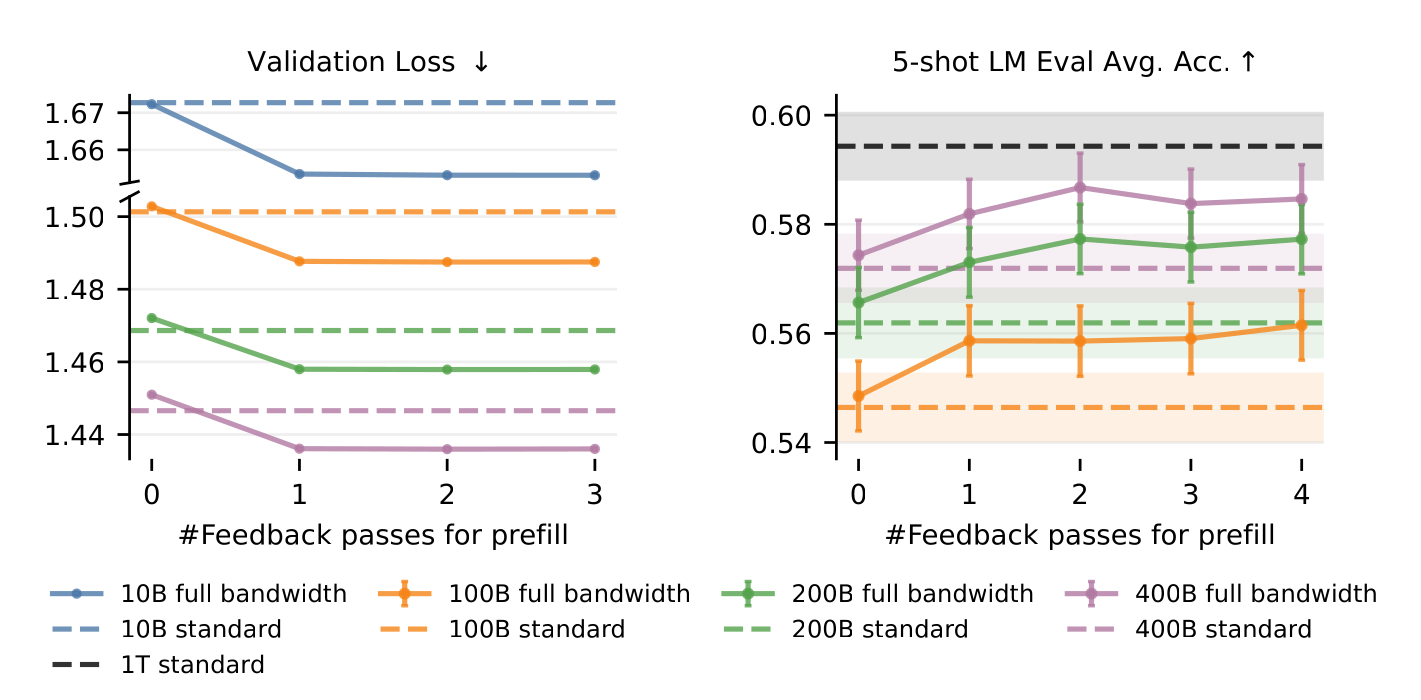
Extra passes over the prompt (§4.1, Figure 5). Feedback passes are run over the prompt before the loss or the answer is read off. “Broadly, most of the improvement appears after the top-layer hidden states are first made available at the input. Further passes continue to help, but with diminishing returns.” Against larger baselines: “With two feedback passes, the 100B-token full-bandwidth transformer reaches the 200B-token standard baseline”, and the 200B model is said to reach the 400B baseline in the same way. With no extra pass, the models “give up only a small amount of validation loss relative to the standard baseline, while already improving average LM Eval accuracy”. The text gives no value for any of these.
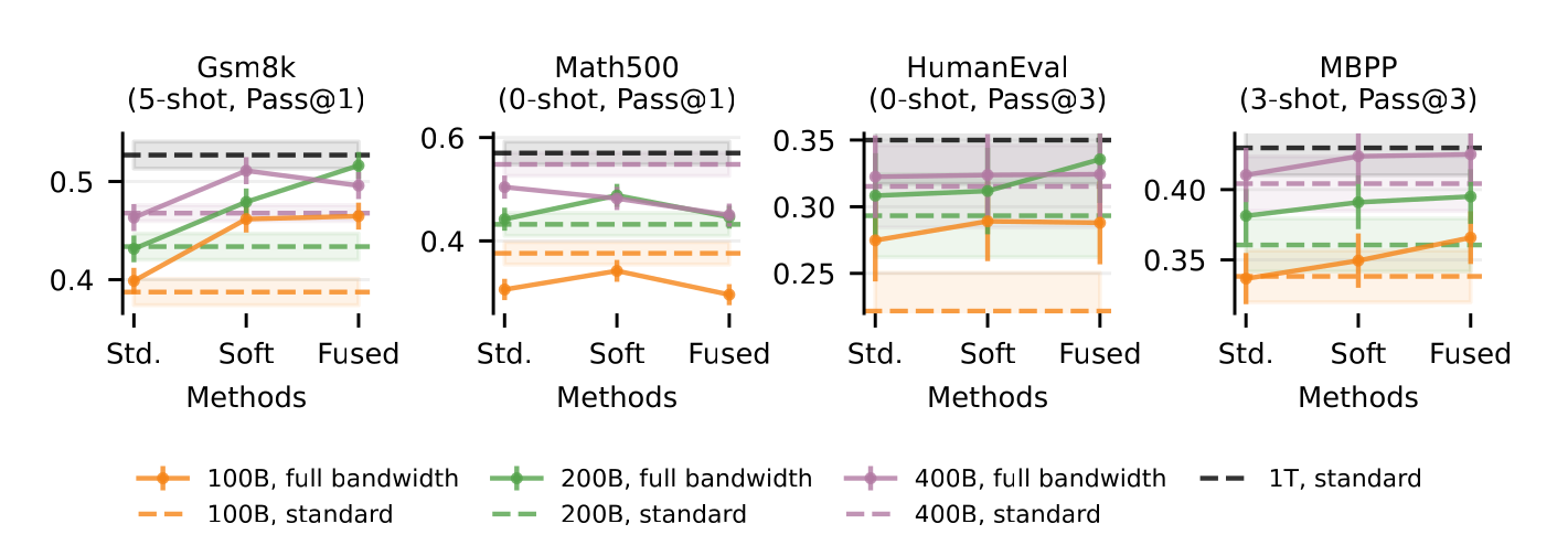
Free-form generation from the pretrained models (§4.2, Figure 6). “Across GSM8K and coding tasks, SOFT generally improves over STANDARD at the same decoding cost, while FUSED can provide further gains with 2× prefill compute.” On those tasks, “full bandwidth models often approach or exceed standard baselines trained with 2–5× more tokens, including the 1T baseline on GSM8K and HumanEval”. One task goes the other way: “MATH-500 is the main exception: before instruction tuning, latent feedback does not consistently improve over STANDARD, particularly at larger scale.”
After instruction tuning (§4.2, Table 2). Each model gets a long-context extension of 12B tokens, from 8K to 32K, and 6B tokens of instruction tuning, and is then evaluated with no in-context examples. Scores are percentages: Pass@1 for the two math tasks and Pass@3 for the two coding tasks.
| Model | Decoding | GSM8K | MATH-500 | HumanEval | MBPP |
|---|---|---|---|---|---|
| Full-bandwidth, 200B | STANDARD | 64.52 | 43.80 | 42.54 | 38.39 |
| Full-bandwidth, 200B | SOFT | 67.93 | 45.60 | 45.06 | 39.80 |
| Full-bandwidth, 200B | FUSED | 67.55 | 45.60 | 45.92 | 41.22 |
| Full-bandwidth, 400B (1.28×) | STANDARD | 67.90 | 46.00 | 46.50 | 40.50 |
| Full-bandwidth, 400B (1.28×) | SOFT | 71.00 | 45.40 | 47.20 | 40.60 |
| Full-bandwidth, 400B (1.28×) | FUSED | 71.80 | 48.40 | 47.60 | 41.70 |
| Full-bandwidth, 400B (1.5×) | STANDARD | 68.08 | 45.40 | 45.69 | 40.23 |
| Full-bandwidth, 400B (1.5×) | SOFT | 70.74 | 49.00 | 46.35 | 41.36 |
| Full-bandwidth, 400B (1.5×) | FUSED | 73.09 | 48.80 | 48.77 | 42.34 |
| Standard, 200B | 62.93 | 42.40 | 37.16 | 38.61 | |
| Standard, 400B | 68.39 | 46.40 | 44.85 | 40.28 | |
| Standard, 1T | 70.13 | 47.40 | 50.01 | 41.93 |
The paper’s summary of the table: “the best latent-feedback regime outperforms the matched-token standard baseline on all four tasks at every reported scale”, and “the MATH-500 degradation observed in the base models disappears after instruction tuning”. One comparison with the largest baseline is picked out: “At 400B (1.5×), SOFT also exceeds the 1T-token standard baseline on MATH-500 (49.0 vs. 47.4).”
Length (§4.3, Figure 7). “On the base model and 0-shot setting, SOFT decoding often produces shorter reasoning traces than STANDARD”. The figure is for MATH-500 on the 200B model, and the three 400B runs are shown in Appendix H (Figure 12). Over MATH-500 the median generation is 486 tokens under STANDARD, 467 under SOFT and 471 under FUSED (Appendix I, Table 5). The paper prints two problems with the rollouts of the 200B model under both regimes; in the first, both reach the right answer, and 326 tokens are left out of the standard rollout as printed (Figure 21, Appendix P). The authors read the shorter traces as the widened channel at work: “Intermediate computation that would otherwise need to be represented through generated tokens may instead be carried in the recurrent hidden state, reducing the number of tokens needed to reach an answer.”
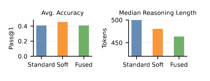
- Objections it expects.
- That training for feedback costs the model when feedback is off. STANDARD decoding is run on every full-bandwidth model to measure this (§4.2), and it is the pass 0 of Figure 5.
- That the baseline is weak. The 200B model is set beside public models of about its size on 0-shot LM Eval, where “we found our model performs on-par or better than models trained under similar or more tokens” (Appendix F, Table 3). “These results imply that full-bandwidth transformers improve on a strong baseline.” (§4.1.)
- That the gain is bought with compute and not with feedback. Table 1 gives each run’s token-equivalent compute, and the comparisons of §4.1 and §4.2 are with baselines trained on two to five times the tokens. In the two post-training stages the full-bandwidth models run three passes throughout, and the baselines get no more data to make up for it: “Baseline standard models are trained on the same set and number of tokens since there is no extra corpus available for spending more compute on.” (Footnote 1.)
- That feeding the state back narrows what the model samples. “Pass@3 improvement on coding tasks suggests that conditioning generation on recurrent hidden states does not reduce sampling diversity” (§4.2).
- That the gain will not survive post-training. This is what Table 2 is for.
- That more prefill passes would give more. “increasing the number of feedback passes for FUSED does not yield further gains” (§4.2), and “the performance does not peak at the number of passes used at training time” (Appendix J, Figure 13).
- That rollouts are far longer than anything the feedback was trained on. They are, and the results stand: “the length is far beyond the three-token horizon the full bandwidth model is exposed to during training” (Appendix I).
- That the shorter reasoning does not last. It does not, and the authors give their guess at why. “Notably, the effect is less pronounced after instruction tuning or given few shot examples.” The examples a model is tuned on or shown were written without feedback: “the target traces were produced by standard token-by-token reasoning, so fitting them re-imposes the fully verbalized style regardless of what the state can carry” (§4.3). Figure 21 says of its example that the difference “is no longer observable on instruction-tuned version”.
- Also reported. On following instructions and on writing the feedback makes no difference. On IFEval and WritingBench, “we did not see full-bandwidth models differ from standard model in these two evaluation settings” (Appendix G, Table 4).
- How strongly it is made. With hedges of how often: SOFT generally improves, FUSED can add to it, the models often approach or exceed. The size of the gain is put three ways. The abstract has “match or approach standard transformers trained with roughly 1.5× more tokens”. The introduction has “the model matches standard transformer baselines trained on twice the tokens in both validation loss and multiple-choice accuracy” (§1). Wang’s first thread has “free-form generation performance comparable with models trained with 2x the FLOPs” (post 6). Langford’s post has no hedge: “Modifying transformer training to support recursive state turns out to be both easy and desirable by all measures.” (his post.) The result on length is the most hedged. The evidence for it is called preliminary (§3.1), and the abstract adds a condition: “when no off-policy templates are provided”.
- What it hands on. The paper’s list of what is not yet shown, below, and a wider frame from the related work: “A promising axis is to spend more computation per unique token through recurrent, iterative, or feedback-based mechanisms.” (§6.)
What the paper claims as new
In its own words, all from §6:
- Against the Feedback Transformer of Fan et al. (2020): “their training is sequential over input tokens, limiting their scalability, whereas our training is parallelized over all positions”.
- Against concurrent work that feeds a late middle layer back into an early one (T²MLR, the Latent Recurrent Transformer, Recirculation): “Our approach mainly differs in the point of reinjection; specifically, our injection happens ‘externally’ to the model and therefore introduces no architecture changes.” And: “We also introduce the least amount of extra parameters.”
- In scale: “our work performs the largest-scale pre-training (up to 400B tokens) among all works, enabled by feedback pass scheduling”.
- Against loop transformers: “full-bandwidth transformer performs recurrence over time, integrated into the autoregressive decoding loop, which avoids additional transformer-block evaluations per generated token”.
- Against latent reasoning methods such as Coconut and Soft Thinking: “(a) We focus on pre-training; (b) We use the hidden state to ‘augment’ the generation rather than replacing the discrete tokens, therefore our approach is easier to supervise (but we may be less token efficient).”
- Against other ways of getting more from the same data: “our framework uses additional training flops for unlocking a new type of decoding regime that gives a free performance boost at inference time”.
The claim is hedged where it meets the nearest work: “we do not foresee reasons why one approach would outperform the others, and exactly which method (and more broadly, which form of past hidden state injection) works the best at large scale remains unclear since we do not have the resources for verification”. Langford’s thread relates the paper to one of those methods, Recirculation: “In essence, the FBT trains for recirculation over the full depth of the stack.” (post 4.)
Limits the authors state
From §7 unless another place is given:
- Scale. “Our experiment scale is limited to 1B parameter models, and we did not verify the approach on models of larger scale.”
- The schedule. It “is based on a heuristic”, and the one given in the main text was unstable at 400B tokens (Appendix E).
- Why three passes are enough is not known (§3.2).
- Depth scaling and weight tying were adopted and not ablated (§3.2).
- The gate. Other fusions did as well in a small test, and the reason given for the asymmetric one found no support there (§3.1, O.1).
- Multi-token prediction. Feedback needs the previous hidden state to produce each next token, so “the current form is incompatible with MTP”.
- Models already trained. Whether a public pretrained model can be turned into a full-bandwidth one is left open: “Future work can further explore the feasibility”.
- Post-training. Scoring rollouts from another policy “can be tricky in off-policy setting”, and the recipes of §5.2 are untested.
- A state that a probe can read is not thereby a state the model uses (Appendix M).
- Sliding-window attention. That feedback could let more layers use a short window is argued and not tested: it “does not recover individual hidden states that have left the window” and offers a compressed path in their place (Appendix K, Figure 14).
- Monitoring. “latent feedback decoding increased the steps of unverbalized compute between two CoT” steps, “therefore increasing the difficulty of CoT monitoring”. The remedy the authors point to: “Future work can consider building probing based monitoring tools that directly reads the hidden states rather than verbal CoT.” Footnote 4 links a discussion of the issue.
How the paper tells it
The paper tells this argument at four lengths: in its title, “Full-bandwidth Transformer”, in the abstract, in the introduction and in the body. This part takes them in that order.
The abstract
Seven sentences. The role is the job the sentence does.
| # | Sentence, abbreviated | Role |
|---|---|---|
| 1 | “Autoregressive transformers compute along two axes: horizontally across generated tokens, and vertically through model depth.” | Context: the frame the title comes from |
| 2 | Attention gives “broad horizontal access to the past, but the vertical feedback channel between decoding steps remains narrow”. | The problem |
| 3 | “We introduce the full-bandwidth transformer, which widens this channel with latent feedback”: the top-layer state fused with the token embedding and fed back. | The contribution, and the mechanism of claim 1 |
| 4 | Feedback “lets non-verbalized computation re-enter the stack with a renewed depth budget, while preserving the standard transformer architecture, KV cache, and language-modeling objective.” | Claim 1: what it gives and what it leaves alone |
| 5 | “we use a scheduled multi-pass objective that introduces latent feedback late in pretraining and mixes a small fraction of deeper feedback passes for stability”. | Claim 2 |
| 6 | 1B-parameter models, up to 400B tokens: “latent feedback improves validation loss, 5-shot language-model evaluation, math and coding generation, and instruction-tuned performance”. | Claim 3: the setting, and the results in words |
| 7 | “match or approach standard transformers trained with roughly 1.5× more tokens”, with shorter reasoning “when no off-policy templates are provided”. | Claim 3: its one number, and the result on length with its condition |
The introduction
Four paragraphs, each with the job it does.
| ¶ | What it says | Role | Cites |
|---|---|---|---|
| 1 | The loop from one decoding step to the next is a channel, and “measured as a communication channel, the loop is narrow”. What is not verbalized is depth-frozen. | The problem, and why it matters | Wei et al. 2022, Li et al. 2024b |
| 2 | The proposal and its name. Two things it affords that standard decoding lacks, and what it costs: “the fusion adds two matrix multiplications per generated token, attention and the KV cache are untouched”. | The approach, and claim 1 | none |
| 3 | “The obstacle is training.” The multi-pass regime, the late schedule, and the finding about three-pass batches. | Claim 2 | none |
| 4 | “full-bandwidth transformers show performance equivalent to substantially more training data”. Prefill, generation, instruction tuning, shorter traces. | Claim 3 | none |
The introduction also carries Figure 1, set between the second and third paragraphs. An unnumbered note on the first page gives the authors’ addresses, says the work was done during an internship, and links the code.
The body, section by section
For each section: its job, how it opens, what it hands on, and what would be missing without it.
§2 Background. Its job is the notation and the frame: the two axes, and equation 2 for what a standard transformer can reach. It ends on the inference the paper rests on, summarized above. Without it the word in the title has no definition.
§3 Widening the bandwidth with latent feedback decoding (claims 1 and 2; Figures 2, 3 and 4). The method, in two halves.
- §3.1 Latent feedback decoding. Opens with the recurrence and the fusion (equations 3 and 4). Then four parts under headings that state their points: it is free to serve, it improves what computation can reach, it adds draft space, and what it does not provide. It hands on a prediction, shorter rollouts, to §4.3.
- §3.2 Parallel multi-pass training for latent feedback decoding. Opens with what the stack sees at decoding (equation 6), and so what it must be trained on. The multi-pass objective (equations 7 to 10), then the schedule, as two questions under their own headings, How many passes and When to introduce feedback passes, then the prefix mixin and the stability measures. It closes by saying which of these were ablated.
Without §3.1 there is nothing to train. Without §3.2 the mechanism cannot be switched on.
§4 Experiments (claim 3; Tables 1 and 2, Figures 5, 6 and 7). It opens with the training setup and Table 1, then one part for each kind of result. §4.1 and §4.2 have their finding as their heading: “Fused prefilling improves non-generative performance” and “Latent feedback decoding improves decoding performance”. §4.3 is the result on length, in two paragraphs. §4.4 is two paragraphs of pointers, to the probes of Appendix M and the ablations of Appendix O. Without §4 the first two claims describe a mechanism with no measured use.
§5 Efficient Replay of Latent-Feedback Trajectories (claim 2; Figures 8 and 9). Its job is to show that the recurrence does not make two routine operations sequential. §5.1 opens with the case: “In actual deployment, a KV cache often needs to be reconstructed from a stored token sequence”. §5.2 opens with post-training and marks itself as hypothetical. Without it a reader is left to ask what happens to a stored conversation and to a rollout from another policy.
§6 Related work. Its job is to set the claim of novelty against what exists, and it comes after the results. Five topics under their own headings: latent recurrence across decoding steps, which opens “One central idea behind our work is to overlap recurrent compute with the sequential decoding process.”; loop transformers; latent and continuous reasoning; parallel training of recurrent networks; and data-efficient pre-training, where footnote 2 links a competition on the question. The last paragraph widens the frame to the axes along which pretraining is scaled.
§7 Limitations and future work. Seven items under their own headings, listed above. Footnote 3 links a public checkpoint that the method could be tried on. The first item ends on a statement of what size cannot buy: the reach the feedback gives “is not something scaling model size or training horizon can acquire”.
Discussion: Origins of the idea. An unnumbered part that closes the main text. “The initial motivation for this work came from observations in NextLat” (Teoh et al., 2025), “where predicting latent states yields a sequence of fixed points, suggesting the feasibility of parallel training a recursive model”. It names the change of view the work came from: “The key shift was to view transformers not merely as fixed-depth feedforward transformations, but as transition operators acting over latent belief states, enabling recursive computation without losing parallelizability.” Langford’s thread gives the same origin with one more source: the proof in the NextLat paper “implies convergence to a sequence of fixed points”, and after the ParaRNN paper “it was clear how to efficiently train a parallel traversal of a set of fixed points” (post 3).
The appendices
Each by the job it does.
| Appendix | Holds | Job |
|---|---|---|
| Appendix A | The architecture of the 1B model | Detail to replicate |
| Appendix B | How the top-layer state is kept for each request under vLLM | Detail of the implementation |
| Appendix C | Figure 10: the training and inference code with the two RMSNorms and the noise | Detail to replicate |
| Appendix D | Seconds per training iteration at one to four passes | Cost of training |
| Appendix E | Five panels: three schedules at 200B and 400B tokens, 1,000 passes, and the 400B results for each schedule | Check: the schedule at larger scale, where it fails |
| Appendix F | Table 3: 0-shot LM Eval beside public models of about 1B parameters | Check: the baseline is strong |
| Appendix G | Table 4: IFEval and WritingBench | Extra result: no difference |
| Appendix H | Figure 12: accuracy and reasoning length for the 200B run and three 400B runs | Check: other runs |
| Appendix I | Table 5: generation lengths by task and regime | Check: rollouts far longer than the training horizon |
| Appendix J | Figure 13: FUSED with up to 11 extra prefill passes | Check: more passes |
| Appendix K | Figure 14: feedback under sliding-window attention | Argument for future work |
| Appendix L | Table 6: throughput and latency under vLLM | Check: the cost of serving |
| Appendix M | Figure 15: probes at every depth on three synthetic tasks | Check: the state arrives at layer 0 |
| Appendix N | The synthetic tasks and the probes in full | Detail to replicate |
| Appendix O | Detached states, other schedules, the gate’s matrices, training curves, the noise: Figures 16, 17, 18 and 19 | Checks on the design |
| O.1 | Figure 20: three fusion gates on a 20-layer Nanochat model | Check: the form of the gate |
| Appendix P | After Figure 21, a second problem with its rollouts under both regimes | Examples |
The same three claims at every length
Where each claim appears, from the shortest statement of the paper to the longest, then in the authors’ threads:
| Where | Claim 1 | Claim 2 | Claim 3 |
|---|---|---|---|
| Title | “Full-bandwidth Transformer” | ||
| Langford’s post | “Modifying transformer training to support recursive state turns out to be both easy” | “desirable by all measures” | |
| Wang’s first post | “we feed previous hidden state into the input together with token embedding” | “it boosts performance for free” | |
| Figure 1, caption | “This returns full hidden-state information to the bottom of the stack” | ||
| Abstract | sentences 3–4 | sentence 5 | sentences 6–7 |
| Introduction, §1 | paragraph 2 | paragraph 3 | paragraph 4 |
| Section | §2, §3.1 | §3.2, §5 | §4 |
| Main-text figures and tables | Figures 1 and 2 | Figures 2, 3, 4, 8 and 9, Table 1 | Figures 5, 6 and 7, Table 2 |
| Wang’s thread | posts 2–3 | post 4 | posts 5–6 |
| Wang’s thread on the revision | post 4 | posts 2, 3 and 5 | |
| Langford’s thread | posts 3–4 |
Wang’s first thread was posted with the paper’s first version, and the images on it carry that version’s numbering: the prefill result as Figure 4, the generation result as Figure 5 and the instruction-tuning table as Table 1. The images on his second thread are the paper’s Figures 18, 1, 8 and 20, a chart of an RL run that is not in the paper, and the closing discussion.
Threads
- Xi Wang on the revision of "Full-bandwidth Transformer" The lead author lists in six posts what the paper's second version adds: how to debug a training run from its loss curves, rebuilding a rollout's KV cache and hidden states with three parallel passes, other forms of the fusion gate, and where the idea came from. One post reports a first online RL run on the released code, which the paper does not contain.
- John Langford on where "Full-bandwidth Transformer" came from Asked about a rumor that a model from OpenAI uses a full-bandwidth transformer, the senior author says in five posts that he has no special knowledge and that, if it is true, it is a case of parallel development. He gives where the idea came from: a talk at NeurIPS that named recursion as a next step, the proof in the NextLat paper and the ParaRNN paper. He names two surprises in building it, that NextLat is not needed and that it worked easily, and relates the paper to Recirculation.
- John Langford on "Full-bandwidth Transformer" The senior author quotes the lead author's thread and gives the paper in one sentence: modifying transformer training to support recursive state turns out to be both easy and desirable by all measures.
- Xi Wang on "Full-bandwidth Transformer" The lead author walks through the paper in eight posts: feeding the previous top-layer hidden state back into the input with the token embedding, what that opens across depth, why it costs almost nothing at inference, the multi-pass training it needs and the schedule that keeps the extra cost near 30% of the flops, the gain from extra prefill passes, and free-form generation comparable with models trained with twice the flops. Posted with the paper's first version: the figure and table numbers in the images are that version's.
BibTeX
@misc{wang2026,
  title = {{Full-bandwidth Transformer}},
  author = {Xi Wang and Ziyang Cai and Zheng Zhan and Harry Dong and Ying Fan and Gustavo de Rosa and Tim Pearce and John Langford},
  year = {2026},
  howpublished = {arXiv},
  eprint = {2608.08888},
  archivePrefix = {arXiv},
  url = {https://arxiv.org/abs/2608.08888}
}