Paper · adjacent
Almost Free State Prediction Separation
A prediction stream that writes no keys or values, the free pause token, lowers a 1B Transformer's next-token loss by 0.028 nats at equal tokens and adds no context length, cache or decode steps at inference. Four changes to training cut its cost from about 1.9 times the pretraining FLOPs to 1.33 times the wall-clock with 94% of the gain kept, and to 1.09 times with less of it, and the two-pass schedules stay ahead of the control at equal node-hours by 0.005 to 0.013 nats.
AI-drafted summary, not yet reviewed by a person. Written from: full text (arXiv v4), appendices included; the thread of one of the two first authors.
The paper in brief
- Problem. State–prediction separation lowers a language model’s loss by running a second stream through the network. “The separation works, but it is expensive: the prediction stream is a second pass over the whole backbone, costing ∼1.9× the pretraining FLOPs, and even more in terms of wall-clock time when using a flexible attention mask.” (Abstract.)
- Why it matters. “even a small but reliable reduction in next-token loss is valuable provided it does not cost the parameters, tokens, inference budget, or training compute that would negate it.” Training compute is the hard one: “an architectural change that improves loss but doubles the cost of pretraining is not an improvement at all, because the older architecture training with more tokens may be superior”. (§1.)
- Question. The authors measure what each of their changes saves, “and then ask whether the gain survives once the control is handed the compute the separation would have consumed.” (§6.)
- Answer. Within one model size and one seed, “state–prediction separation provides a modest iso-token/parameter/compute/training FLOP advantage over standard pretraining methodology.” The cost that made it “an expensive curiosity” falls “to 1.33× wall-clock with essentially all of the gain intact, and to as low as 1.09× if some is traded away, while inference stays free.” (§7.)
The three claims are a chain. The first is the mechanism and what it gains when both models see the same tokens. The second is what the mechanism costs to train and how that cost is cut. The third puts the two together: with the cost that low, the gain is still there when the control is given the same compute.
- A prediction stream that writes no keys or values, the free pause, lowers a standard Transformer’s next-token loss at equal tokens and adds nothing to the sequence at inference.
- Four changes to training cut the cost of that second stream from about 1.9× the pretraining FLOPs to 1.33× the wall-clock with nearly all of the gain kept, and to 1.09× with part of it given up.
- At equal compute the free pause is still ahead of the control, and the cheapest schedules are ahead by the most.
What the paper starts from
The two burdens (§1). A decoder Transformer predicts the next token from the hidden state at the current position. “That single state carries two burdens at once”: it must summarize the context so far, which is “the state that later positions attend to”, and it must be a good predictor of the next token. “These two goals pull in different directions, yet a model with one state per position must serve both from the same vector.”
State–prediction separation, SPS for short. The hypothesis and the architecture that tests it come from Monea et al. (2026): “the forward pass is split into a state stream and a prediction stream so that summarizing and predicting need not share one representation” (§3). The two streams run over one set of weights, and the loss comes down. The price is the second stream: “a prediction stream is a second pass over every layer, so SPS asks for roughly 1.9× the pretraining FLOPs of the model it improves” (§1).
Terms.
- State stream, written a: the ordinary forward pass, “which summarizes the context and exposes per-layer keys and values” (§1).
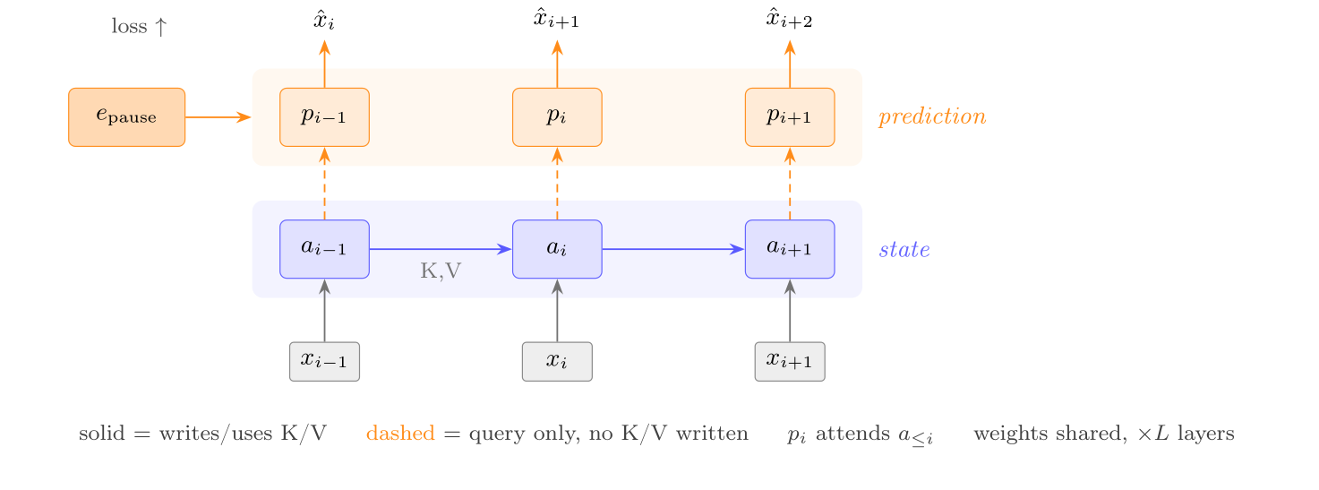
- Prediction stream, written p: “At every position p starts from one learned embedding, forms a query at each layer over a’s keys and values, and emits the next-token prediction; the training loss falls only on p.” (§1.)
- Free pause token, or free pause: the prediction stream in the form this paper gives it, in which it “writes no keys or values of its own, so it adds nothing to the sequence” (§1).
- w, the prediction window. In the earlier architecture “the prediction stream still writes keys and values that are retained within a sliding window of w tokens”. The free pause “is the w=0 limit taken strictly: the prediction writes nothing at all, forming only a query over the state’s keys and values” (§3).
- Pause token (Goyal et al., 2024): a learned position inserted into the sequence, “giving the model extra forward passes to ‘think’ before it commits” (§3). It is the thing the free pause is named for and set against.
- Full pause, and phased. A full pause trains with the prediction stream from the first step. A phased run trains as a standard Transformer first and switches the stream on partway; the tables name such a run by the share of the tokens trained the standard way, 42.5% or 75% (§2, Table 2).
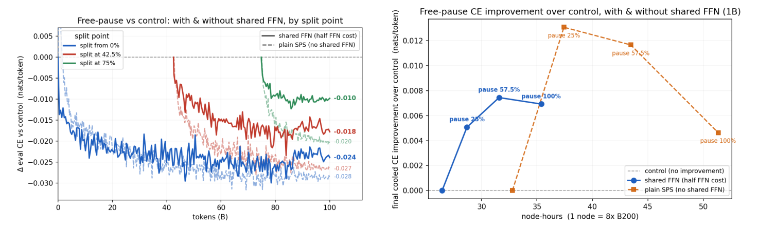
- Cooled. The learning rate ends each run with “a final-25% linear cooldown” (§4), and the loss the paper compares is the one at the end, the “final cooled CE” of Figure 1.
The mechanism (§2, Figure 2). At every position and every layer the prediction stream reads the state stream’s keys and values up to that position and writes none back. The streams share every weight: “Because every backbone parameter is shared, the model differs from a standard Transformer by exactly one tensor” (§2). That tensor is the learned vector the prediction stream starts from at every position, predict_embedding in the text and e_pause in the figure.
The inference it rests on (§1). Next-token cross-entropy “is known to track downstream capability closely enough to anchor the scaling laws that govern modern pretraining”, so a lower loss is worth having. A control can also buy a lower loss, with more tokens. So a gain counts only against a control that was given the same resources, and the paper names four: parameters, tokens, inference budget and training compute.
The setting (§4). One model: “A 1B decoder transformer: 24 layers, hidden size 1536”, with a sequence length of 8192, pretrained on “Phi-4 derived data” with a global batch of 524,288 tokens on 8×B200. The runs compared are trained on 100B tokens. The control is “the identical model with the prediction stream removed, matched on optimizer, data order, schedule, and global batch, so the two differ only in the second pass—and hence in wall-clock throughput”.
- Quality is the eval cross-entropy of next-token prediction, in nats per token; lower is better, and a centinat is a hundredth of a nat.
- Cost is time on fixed hardware: “Compute is reported as wall-clock node-hours on identical 8×B200 hardware—the cost actually paid.”
- Three comparisons follow from these. Iso-token: both models have seen the same number of tokens. Iso-compute: both have had the same node-hours, so the control has seen more tokens; “iso-compute below means iso-node-hours which account for the higher utilization”. Iso-FLOP: both have had the same floating-point operations, which is stricter, because the second pass costs more in FLOPs than in time.
- Downstream, two pooled measures: DCLM CORE, “a centered mean over 21 multiple-choice tasks”, and bits-per-byte on held-out text from climbmix.
What the design rules out.
- A gain that comes from some other difference in training. The control shares the optimizer, the data order, the schedule and the batch (§4).
- A gain bought with parameters. “the only added parameter is e_pause” (Figure 2).
- A cost that an operation count would misstate. The second pass runs the hardware at a different utilization than the control does, so cost is measured as time on the same machines (§5).
Tools taken from earlier work. The separation itself (Monea et al., 2026). Pause tokens (Goyal et al., 2024). FlashAttention kernels (Dao et al., 2022), in the version written for Blackwell GPUs (Zadouri et al., 2026). A Muon-family optimizer (Jordan et al., 2024). Pretraining data derived from Phi-4 (Abdin et al., 2024). For the downstream measures, DCLM CORE (Li et al., 2024), climbmix (Diao et al., 2025) and lm-eval (Gao et al., 2023). For serving, vLLM (Kwon et al., 2023).
The argument, claim by claim
Claim 1: a prediction stream that writes nothing lowers the loss at equal tokens and is free at inference
The free pause lowers a standard Transformer’s next-token loss when both are trained on the same tokens, and it adds no position, no cache entry and no decode step when the model is run.
Evidence. At equal tokens, “the free pause reaches 2.8673 versus the control’s 2.8957—a −0.0284 nats iso-token gain” (§6). The abstract gives the size of the gain as “2-3 centinats in practice on a 1B parameter model”.
At inference the argument is from the design, with one measurement (§6.4). To read a prompt, only the state stream runs, “so the cost is the same as a vanilla Transformer”. To generate, the token and its prediction “forward together as a two-token step”, which “adds only the prediction stream’s parallel compute within each step—extra FLOPs, not extra depth”. The measurement is a microbenchmark of one decode step on B200, in which batching the two streams and sharing the cache read “puts the fused free-pause decode step within ∼1% of a standard decode” (Appendix A).
Downstream, at equal tokens, “the full pause raises DCLM CORE from 0.327 to 0.347” and lowers bits-per-byte on climbmix from 0.777 to 0.769 (§6.5, Table 5). The whole of Table 5 is under claim 3, which uses its other rows.
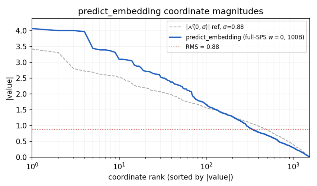
- Also reported: what the one new tensor learns (§6.6, Figure 5). The embedding grows during training “but is RMS-normalized before use, so only its direction matters”. “That direction leans modestly toward the frequency prior. The nearest tokens by cosine are the commonest continuations”: comma, period, newline, the and and, at cosines of 0.25 to 0.46. About a dozen coordinates stand well above the rest and carry “∼11% of the energy over a diffuse bulk”. Set against the table of token embeddings, “it is a distinct, atypical point”. No claim rests on this section.
- Objections it expects.
- That the gain shows in the loss and nowhere else. §6.5 opens with it: “Does the per-token gain survive as downstream capability, or is it loss-only?” The two pooled measures are the answer, and they are pooled because single tasks cannot show it: “task scores are within their 95% confidence intervals so relevant signal is in these pooled and dense measures”. The section concludes: “The gain is therefore not a loss-only artifact: it appears in downstream compression and in aggregate task accuracy.”
- That a second stream cannot be free to run, since it computes more. The paper grants the operations and argues that they do not set the speed: “It is very typical for autoregressive latency to be set by the decode’s sequential depth (one step per generated token, L layers each), which the free pause leaves unchanged.” (§6.4.) The abstract says the same of throughput, calling “the growth in inference flops typically irrelevant as it is not the active bottleneck on throughput”.
- That one run is noise. “in our experience the pretraining process is robust enough that the results reported here are beyond the noise level” (§7).
- How strongly it is made. As a small gain: “modest benefit consistent with the −0.028 nats CE gain” (§6.5). And free is qualified wherever it is spelled out: “effectively free at inference” and “near-free decode latency” (§1), “essentially no latency” (Abstract).
- What it hands on. A cost that is all on one side. “The primary remaining issue is therefore just training cost.” (§1.)
Claim 2: four mechanisms cut the training cost of the second stream
The free pause is paid for in training, where the prediction stream is a second pass over the layers. Four mechanisms bring that from about 1.9× the FLOPs of standard pretraining to 1.33× its wall-clock with nearly all of the gain, and to 1.09× with part of it.
The starting point is fixed in §5. The second pass reuses the state stream’s keys and values, “implying a cost of ∼1.9× FLOPs, not 2×”. In time it is less: “Its wall-clock overhead is lower still (∼1.57×), because the compute-dense pass runs at ∼20% higher utilization than the micro-batch-4 baseline.” So 1.57× the control’s node-hours is what a full pause costs when run as two passes, and Table 1 measures the mechanisms against that figure.
Evidence. One mechanism at a time, in the paper’s order.
- A two-pass split that stock attention kernels can run (§2, §6.1). Because the prediction stream writes nothing, training can run the state stream first and then the prediction stream “as a plain cross-attention over them”. FlashAttention kernels handle both shapes, and they do not handle the mask of the interleaved form, which is “neither causal, sliding-window, nor block-diagonal over packed sequences”. The measurement: “73k tokens/s per GPU instead of 16k tokens/s with a single pass flexible attention mask, about a 4× improvement” (§2).
- No window for the prediction stream, w = 0 (§6.1). The earlier architecture kept a small sliding window among the prediction stream’s own keys and values. Here “the prediction self-window helps by only −0.0047 with 100B tokens”, and keeping it “needs a second, log-sum-exp–merged FA call increasing compute by 1.22× the w = 0 pass”. The two runs behind the first figure are in Appendix B: 2.8626 with a window of 64, and 2.8673 with none.
- A shared gated FFN (§2, §6.2). The feed-forward layers hold most of the parameters, so they are most of the second pass. A scalar gate per token pools the two streams’ inputs, “a single FFN is applied to the pooled input, and two further scalar gates route its output back into each stream”. “One FFN evaluation per position thus replaces two.” Peak memory falls by about 14 GB per GPU, “91 vs 105 GB at micro-batch 4”, which is “enough that it fits a larger, faster micro-batch on which the two-pass form OOMs”. Throughput rises from 0.64× the control’s to 0.74×, and so “A full pause therefore costs 1.35× control wall-clock rather than 1.57×”. The quality is in Table 3, given below, and the paper’s reading of it is that the shared form “still beats the control at every split point” but “gives up some of the two-pass form’s advantage (∼0.005–0.010 nats/token), so there is a real cost associated with the shared FFN”.
- Phasing (§2, §6.1). “Training runs as for a standard next token prediction transformer for a fraction f of the schedule and switches on the split for the remainder”. The second pass is then paid on the rest of the tokens only, and §2 gives the compute as f + (1 − f) · 1.57. This is possible because the model has the same parameters as a standard one, so that “a standard checkpoint is already a valid backbone” (§2). The results are in Table 2, given below.
Phasing first, in the two-pass form (Table 2). The last column is the paper’s: the loss given up against the full pause, and the share of the full pause’s gain that is kept.
| Schedule | CE at 100B | Compute | Against the full pause |
|---|---|---|---|
| Control, no pause | 2.8957 | 1.00× | |
| Full pause, w = 0 | 2.8673 | 1.57× | |
| 42.5% standard, then pause | 2.8691 | 1.33× | +0.0018, recovers 94% |
| 75% standard, then pause | 2.8756 | 1.14× | +0.0083, recovers 71% |
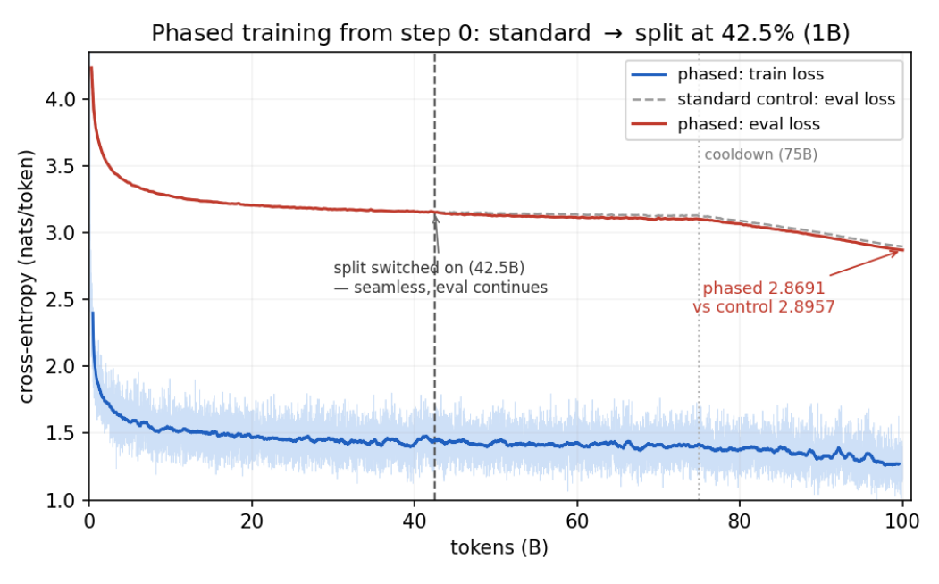
“Switching to the pause at 42.5% recovers essentially all the gain (2.8691, within noise of full pause’s 2.8673) at 1.33× instead of 1.57×” (§6.1). The switch does not disturb the run: “the phased run tracks the control’s loss up to the switch—the switch is seamless, no visible spike—then diverges below it and cools to 2.8691” (Figure 3).
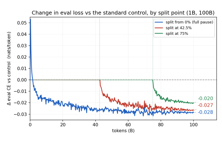
How late the switch can come is the subject of Figure 1’s left panel. “a cold start with the full pause is actually worse for training of ∼1.5B tokens but then provides a clear win”, and “Most of the benefit accrues within ∼15B tokens of free pause training although small gains continue to be observed the longer free pause training continues.” The paper’s conclusion from the shape: “late phase free pause token training achieves most of the gains of early phases for a small fraction of the overall compute”. (§6.1.)
Then the shared gated FFN, alone and with phasing (Table 3). These runs use a faster micro-batch, so they have a control of their own, and the change is against that control.
| Schedule, shared FFN | CE at 100B | Change | Compute |
|---|---|---|---|
| Control, no pause | 2.9064 | 1.00× | |
| Full pause, w = 0 | 2.8825 | −0.0239 | 1.35× |
| 42.5% standard, then pause | 2.8886 | −0.0178 | 1.20× |
| 75% standard, then pause | 2.8966 | −0.0098 | 1.09× |
The last row is “the cheapest point in the paper” (§6.2).
All four together, in the abstract’s words: “Together these bring the overhead versus an optimized pretraining pipeline to 1.33× wall-clock while recovering ∼94% of the gain compared to SPS, and to as low as 1.09× along a graceful quality/compute tradeoff.” Langford’s thread gives the saving in other figures: “The training time overhead is reduced from ~700% in SPS to an amortized 10-20% depending on precise choices.” (post 2.)
- Objections it expects.
- That switching architecture in mid-run upsets training. In the two-pass form nothing is reset: “step, schedule, backbone optimizer, and dataloader all continue; only predict_embedding initializes fresh” (§2), and Figure 3 shows no spike. Of the shared FFN the paper says the opposite: “The switch is not fully function-preserving”, and so “unlike the two-pass form it requires some training to settle after the switch” (§2).
- That a late switch leaves the pause no time to learn. “The 75% split (1.14×) tests the hard case where the pause gets only the cooldown to adapt.” (§6.1.) It keeps 71% of the gain.
- That the shared FFN changes the model, so that a standard checkpoint no longer fits. “No backbone parameter changes, so a standard checkpoint can still be phased in.” The three gates are “single-output linears (negligible parameters)”. (§2.)
- That the shared FFN’s loss is being read against the wrong baseline. “Part of that apparent gap is a baseline artifact: to fit the faster micro-batch the shared runs use a slightly smaller global batch whose own control is ∼0.011 nats/token worse, so the iso-batch cost of sharing is smaller than the raw deltas suggest.” (§6.2.) Table 3 and the right panel of Figure 4 set each form against its own control.
- How strongly it is made. With the price of each step stated beside it. The 1.33× comes “with essentially all of the gain intact”, and the 1.09× only “if some is traded away” (§1). The 42.5% schedule is “within noise” of the full pause (§6.1), and the shared FFN has “a real cost” (§6.2).
- What it hands on. A cost in node-hours for every schedule, which is what a comparison at equal compute needs.
Claim 3: at equal compute the free pause is still ahead, and the cheapest schedules by the most
Give the control the node-hours the second pass used, to spend on more tokens, and the free pause still has the lower loss. The margin is largest for the schedule that spends the least on the pause.
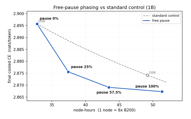
Evidence. “At iso-compute the baseline spends the saved node-hours on extra tokens; the comparison is the pause at 100B against the control given the same node-hours” (§6.3). The control was run to 100B and to 150B tokens, ending at 2.8957 and 2.8742 (Appendix B), from which the paper takes a slope of “∼0.037 nats/doubling” (Table 4). The control’s loss at other token counts is read off that line: “114–133B interpolated, 157B a short extrapolation”. Table 4, with the control’s loss at equal node-hours in the fourth column:
| Schedule, two-pass | CE at 100B | Compute | Control at equal compute | Margin |
|---|---|---|---|---|
| Full pause, w = 0 | 2.8673 | 1.57× | 2.872, at 157B | −0.005 |
| 42.5% standard, then pause | 2.8691 | 1.33× | 2.881, at 133B | −0.012 |
| 75% standard, then pause | 2.8756 | 1.14× | 2.889, at 114B | −0.013 |
“Every free-pause variant is ahead at equal node-hours.” (Table 4.) And the order of the rows is the paper’s point: “Note the ordering: the cheapest schedules are the ones that win most at equal compute, which is precisely the point of making the separation almost free rather than merely effective.” (§6.3.)
The right panel of Figure 1 draws the same comparison as two curves. The introduction reads it: “plotted against wall-clock node-hours the resulting frontier stays below the control’s own compute-for-loss curve, so the gain survives at equal compute—an iso-compute improvement” (§1). And §6.1 reads its shape: “a short pause finish banks most of the gain per extra node-hour”.
Downstream, the comparison at equal compute is with the control trained on 150B tokens (§6.5, Table 5).
| Run | DCLM CORE, higher is better | Bits-per-byte on climbmix, lower is better |
|---|---|---|
| Control, 100B | 0.327 | 0.777 |
| Control, 150B | 0.348 | 0.770 |
| Full pause, w = 0, 100B | 0.347 | 0.769 |
| 42.5% standard, then pause, 100B | 0.348 | 0.769 |
| 75% standard, then pause, 100B | 0.348 | 0.771 |
The standard error is about 0.01 on DCLM CORE and about 0.004 on bits-per-byte (Table 5). The paper’s reading: “Iso-compute, the pause at 100B matches the control given 50% more tokens (150B) to within measurement error on both metrics, and phasing reaches the same level at 1.14–1.33× compute.” (§6.5.)
- Objections it expects.
- That time on the clock flatters the pause, whose second pass runs the hardware harder. The answer is the stricter count, and the paper reports the case it loses: “The margins tighten with a stricter iso-FLOP (∼1.9×) analysis where the phased runs stay positive (−0.005 to −0.009) while the full pause turns slightly negative (+0.006).” (§6.3.)
- That the control’s loss at 114B, 133B and 157B was never measured. It is taken from two endpoints that were, and Table 4 says which of the three is beyond them.
- That the size of the win depends on the accounting. The paper says so: “a clear and desirable compute win of ∼1 centinat depending on how measurements are done” (§6.3).
- How strongly it is made. Most strongly where it is shortest: “The result is an isoflop, isoparameter, and isotoken improvement over standard next token trained transformers.” (Abstract.) Under Figure 1 it has a range, “improvements over standard control vary from −0.005 to −0.013 nats”. In the conclusion the separation “provides a modest” advantage, and the sentence that says so comes after its scope: “Our experiments here are limited to a single scale (1B) with a single primary seed.” (§7.)
- What it hands on. Two combinations left untried. With speculative decoding, which uses the same spare compute at inference: “We leave investigating the combination of both techniques here to later work.” (§3.) And with predicting several tokens at once: “One perhaps-significant variation that may matter in practice is combining this approach with multitoken prediction” (§7).
What the paper claims as new
In its own words:
- The mechanism. “We take state–prediction separation to its limit with a free pause token, which gives the prediction its own computation without a sequence position.” (§1.)
- Against the earlier architecture. “This stricter separation is what makes the method free at inference since the prediction adds no cache. It is also what makes the training cheap” (§3).
- Against pause tokens. “the free pause delivers the effect of a pause token” and does so “without spending a sequence position on it” (§1).
- Against speculative decoding. “A free pause token leverages exactly the same spare compute which speculative decoding benefits from for the purpose of improving prediction quality rather than prediction speed.” (§3.)
- Against work done at the same time. Decode-Branch Transformers (Liu et al., 2026) “aims at a similar idea”. The differences the paper names are “the phasing optimization here” and “the broader study of Mixture of Experts models there”, and it takes the two together as support: “these results reinforce the value and scope of free pause tokens”. (§3.)
- In Langford’s thread. The paper is State Prediction Separation run “through an optimization process”, “finding that it works at higher op and yielding ‘free pause tokens’ which allow a transformer to make higher quality inference for (near) free” (post 1).
Limits the authors state
- One size and one seed: “a single scale (1B) with a single primary seed” (§7).
- At equal FLOPs the full pause loses to the control, and the phased margins shrink: “the full pause turns slightly negative and the phased deltas roughly halve, though the ordering is unchanged” (§5).
- The control’s loss at equal compute is partly interpolated and, for the full pause, extrapolated (Table 4).
- Single downstream tasks do not separate the models: “Per-task lm-eval scores are individually within their 95% intervals and are not shown.” (Table 5.)
- The shared gated FFN costs quality (§6.2), and its switch is not function-preserving (§2).
- A full pause from a cold start is behind the control for the first 1.5B tokens or so (§6.1).
- Inference is not free in operations. The prediction stream adds “extra FLOPs, not extra depth” (§6.4).
How the paper tells it
The paper tells this four times, each longer than the last: in its title, “Almost Free State Prediction Separation”, in the abstract, in the introduction and in the body. This part takes them in that order.
The abstract
Nine sentences. The role is the job the sentence does.
| # | Sentence, abbreviated | Role |
|---|---|---|
| 1 | SPS “relieves a language model’s hidden state of two competing burdens” by splitting the forward pass into two streams. | Context: the earlier idea |
| 2 | “The separation works, but it is expensive” | The problem, with its number |
| 3 | “This paper makes state–prediction separation almost free.” | The contribution, in the title’s words |
| 4 | “a free pause token: a prediction stream that writes no keys or values at all and so rides the sequence’s existing positions” | The mechanism |
| 5 | It improves prediction “by 2-3 centinats in practice on a 1B parameter model”, and “because it adds no position it costs nothing at inference”. | Claim 1, with its number and a hedge on inference FLOPs |
| 6 | “The cost is therefore entirely in training where we use four mechanisms to drive it down” | The turn to claim 2, and the four mechanisms named |
| 7 | Overhead of “1.33× wall-clock while recovering ∼94% of the gain”, and “as low as 1.09×”. | Claim 2, with its numbers |
| 8 | “the FFN optimization reduces the raw flops required at inference time” | A further benefit |
| 9 | “The result is an isoflop, isoparameter, and isotoken improvement” | Claim 3, and the close |
The introduction
Six paragraphs, each with the job it does.
| ¶ | What it says | Role | Cites |
|---|---|---|---|
| 1 | Next-token loss tracks capability, so “even a small but reliable reduction” is worth having, unless it costs what would cancel it. Training compute is the hard case. | Context, and the test any result must pass | Kaplan et al. 2020, Shannon 1951, Delétang et al. 2024, Hoffmann et al. 2022 |
| 2 | One hidden state has two jobs. SPS gives each its own stream and lowers the loss, at roughly 1.9× the FLOPs and more on the clock. | The earlier idea, and its problem | Monea et al. 2026 |
| 3 | “We take state–prediction separation to its limit with a free pause token”. What the two streams do, and why the pause costs nothing at inference. | The mechanism and claim 1, ending on the handover to claim 2 | none |
| 4 | “We drive this cost down using four mechanisms, all developed in §2.” First to fourth, then the figures 1.33× and 1.09×. | Claim 2, as a numbered list | Dao et al. 2022, Zadouri et al. 2026 |
| 5 | Where the work sits, beside pause tokens and speculative decoding. The evaluation: one 1B model against “a tightly matched control”. | Positioning and setup, as pointers to §3 and §4 | Goyal et al. 2024; Cai et al. 2024, Chen et al. 2023, Leviathan et al. 2023, Stern et al. 2018; Abdin et al. 2024 |
| 6 | “Figure 1 previews the payoff at the cheap end of that range.” A lower loss at every point in training, and a frontier under the control’s. | Claim 3, by pointing at a figure | none |
The introduction carries both of the paper’s leading figures. Figure 1 is on the title page, under the abstract. Figure 2, the mechanism, is set between the fifth paragraph and the sixth.
The body, section by section
For each section: its job, how it opens, what it hands on, and what would be missing without it.
§2 Method. Its job is to define the mechanism and the changes to training that need defining. It has four paragraphs, each under a heading of its own: the two streams, the two-pass split, the shared gated FFN and phasing. It opens “Concretely”, picking up the introduction’s sketch, and the first paragraph ends by naming what a later one will use: “the property phasing exploits below”. The paragraph on the shared FFN hands on to the results: “The FLOP, memory, and quality consequences are measured in §6.2.” Without this section the gates of the shared FFN and the cost formula for phasing are nowhere in the paper.
§3 Related work. Its job is to say what is new against four neighbors, and it comes before the results. One paragraph each: the earlier architecture, pause tokens, speculative decoding and one parallel effort. Each ends by placing the free pause against the work it describes. It is also where w = 0 is defined, and the one place that says how the free pause differs from the earlier architecture at the same setting, which “also writes a temporary key and value for the prediction stream”.
§4 Model and optimization. Its job is to fix everything the runs share: the architecture, the optimizer and schedule, the data and the control. Three short paragraphs. Without it the word matched, said of the control, has no content.
§5 Measurement. Its job is to say what cost means: 1.9× in FLOPs, 1.57× on the clock, and node-hours as the unit of the tables. Its last sentence gives a result ahead of the results, the outcome at equal FLOPs. Without it the compute column of every table is unreadable.
§6 Results. It opens with the headline number and one sentence of plan, the one quoted as the paper’s question above. Then six subsections:
- §6.1 Cutting the second pass (Tables 1 and 2; Figures 1 and 3). Table 1 comes first, as a summary of the four mechanisms, then a paragraph on each. Most of the text is on phasing.
- §6.2 The shared gated FFN in practice (Table 3, Figure 4). It opens by saying what it is for: “What that buys is measured here.” Memory and throughput, then quality.
- §6.3 Iso-FLOP analysis (Table 4). The comparison at equal compute, closing on the ordering of the schedules.
- §6.4 Inference cost. One paragraph with no table or figure, pointing to Appendix A.
- §6.5 Downstream evaluation (Table 5). It opens with the objection it answers, as a question.
- §6.6 What the pause embedding learns (Figure 5). A description of the one new tensor.
Without §6.3 the title has a cost and no reason to pay it. Without §6.5 claim 1 is a claim about loss alone.
§7 Conclusion. Five sentences. The limits come first, then the claim “Within that scope”, then the cost figures of claim 2 once more, then one direction for later work.
The appendices
Each by the job it does.
| Appendix | Holds | Job |
|---|---|---|
| Appendix A | Engineering: how the two streams are served in vLLM as one batch over one cache, and the decode-step microbenchmark | The measurement behind claim 1’s free at inference |
| Appendix B | Cross-entropy summary: six runs and the loss each ends at, in a table with no number | Reference. The only place that gives the control at 150B, 2.8742, and the pause with a window of 64, 2.8626 |
The same three claims at every length
Where each claim appears, from the shortest statement of the paper to the longest, with the thread’s two posts after the title:
| Where | Claim 1 | Claim 2 | Claim 3 |
|---|---|---|---|
| Title | “Almost Free State Prediction Separation” | ||
| Thread, post 1 | “higher quality inference for (near) free” | ||
| Thread, post 2 | “reduced from ~700% in SPS to an amortized 10-20%” | “an improvement on basic transformers which may be widely useful” | |
| Conclusion, §7 | “while inference stays free” | “fall to 1.33× wall-clock with essentially all of the gain intact” | “a modest iso-token/parameter/compute/training FLOP advantage” |
| Abstract | sentences 4–5 | sentences 6–7 | sentence 9 |
| Caption of Figure 1 | left panel | right panel | |
| Introduction | ¶3 | ¶4 | ¶6 |
| Sections | §6.4, §6.5, §6.6 | §2, §6.1, §6.2 | §6.3, §6.5 |
| Figures and tables | Figures 2 and 5; Table 5 | Figure 1, left; Figures 3 and 4; Tables 1, 2 and 3 | Figure 1, right; Tables 4 and 5 |
Threads
- John Langford on "Almost Free State Prediction Separation" One of the two first authors announces the paper in two posts: state-prediction separation put through an optimization process, which yields free pause tokens that let a transformer predict better at almost no cost at inference, with the training overhead cut from about 700% to an amortized 10 to 20%.
BibTeX
@misc{langford2026,
  title = {{Almost Free State Prediction Separation}},
  author = {John Langford and Nathan Godey and Giovanni Monea and Yoav Artzi and Harry Dong and Ying Fan and Gustavo de Rosa and Zheng Zhan},
  year = {2026},
  howpublished = {arXiv},
  eprint = {2609.03807},
  archivePrefix = {arXiv},
  url = {https://arxiv.org/abs/2609.03807}
}