Paper · adjacent
Finetuning with Sampling: SFT Learns Better Than You Think
arXiv:2610.02140 · project page · PDF · code
A Metropolis-Hastings sampler rewrites expert traces into ones the base model is far more likely to produce while keeping their content, and each of its steps is proved to bring the data closer to the base model in KL divergence. Supervised finetuning on the rewritten data rivals RL and self-distillation, often generalizing better and forgetting less, and the finetuned model's pass@k curve stays above the base model's up to 64 samples, which the authors read as learning beyond sharpening.
AI-drafted summary, not yet reviewed by a person. Written from: full text (arXiv v1), appendices included; the lead author's thread; the lead author's reply to a question about the released code.
The paper in brief
- Problem. “a key open question remains: how can we introduce fundamentally new capabilities during posttraining without giving up existing ones?” (§1.)
- Why it matters. Each of the two standard methods lacks what the other has. Reinforcement learning (RL) is the one credited with generalizing and with keeping what the model already knew, but it “relies on the model’s own ability to find successful trajectories through repeated sampling”, and “This limitation is not ideal for the purposes of introducing new capabilities, where the model is unlikely to already be competent enough to produce a successful trajectory.” Supervised finetuning (SFT) can learn from an expert’s trajectory, but it “suffers from weak generalization and catastrophic forgetting”. (§1.)
- Question. “can we algorithmically sample on-policy trajectories that remain faithful to privileged off-policy information?” (§1.)
- Answer. “this sampling step enables SFT to rival prevailing posttraining techniques, often generalizing better and forgetting less than strong on-policy learning algorithms” (§1).
The three claims are a chain. The first is a method and what is proved of it. The second is what finetuning on its output does. The third answers a doubt the first raises about the second: whether data pulled toward the base model can teach the model anything it could not already do.
- Expert traces can be made on-policy by sampling: the distribution closest to the base model that keeps the traces’ content can be written down, and a Metropolis-Hastings sampler started at an expert trace moves toward it, closer in KL divergence at every step.
- SFT on the data this produces rivals on-policy posttraining, often generalizing better and forgetting less.
- What the finetuned model gains is more than a sharpening of what the base model could already do.
What the paper starts from
Terms.
- Supervised finetuning (§3): minimizing the cross-entropy of the model on a dataset of expert trajectories, each a response to a query (equation 2).
- On-policy and off-policy are used as in reinforcement learning and are not defined. RL is on-policy: “the model’s own samples dictate learning updates”. SFT “is off-policy, leaving finetuning more susceptible to drastic updates and shifts in behavior”. (§1.)
- Catastrophic forgetting: “a phenomenon where finetuned models exhibit significant deterioration in existing capabilities” (§1).
- Privileged information: what the expert trajectories carry. They “provide rich supervision signal without necessitating an explicit reward” (§1).
- Boosted: the paper’s word for a trace, or a dataset, after its sampler has been run on it.
The inference it rests on (§1, §2). Earlier work puts RL’s advantage down to learning on-policy, which keeps the finetuned model close to where it started: “the model’s own samples dictate learning updates, constraining finetuning towards distributions that do not stray far from the original starting point” (§1). One of the works cited, Shenfeld et al. (2025), “even shows that the level of forgetting correlates with the KL divergence of the finetuned model with the base model” (§2). The paper leaves the learning algorithm alone and moves the data: “rather than modifying the learning algorithm to accommodate off-policy data, we ask if we can instead shape the data distribution to accommodate learning” (§1). The step from there to the method is one sentence: “To construct an informational-equivalent dataset that is easiest for the base model to internalize, we must provide a generation policy that maintains this information with minimal KL divergence.” (§4.)
The setting (§5.1). Three tasks, each with expert trajectories “which are either inherent to the dataset or generated by GPT-5”. The base models are chosen to be ones “that are not already proficient or finetuned on the task domains”. The last column is the base model’s accuracy on the task’s test set.
| Task | Data | Expert traces | Base model | Base |
|---|---|---|---|---|
| Chemistry | The Chemistry L-3 subset of SciKnowEval: 2400 problems, 1800 to train on and 600 to test | Generated by GPT-5 | Qwen2.5-7B-Instruct | 34.3% |
| Chemistry | The same | The same | Olmo-3-7B-Instruct | 32.8% |
| Math | MATH, Levels 3, 4 and 5: 9254 problems, 8230 to train on and 1024 to test | The dataset’s own solutions | Qwen2.5-3B | 31.5% |
| Medical | The HuatuoGPT-o1 SFT dataset, 19704 questions; tested on 1000 questions from the HuatuoGPT-o1 RL dataset “that are never seen during training” | The dataset’s own responses | Qwen2.5-7B-Instruct | 35.3% |
Some chemistry questions are multiple choice and others are freeform, “representing a mixed dataset with a harder-to-specify reward for on-policy RL”. Medical answers are graded by GPT-5-mini.
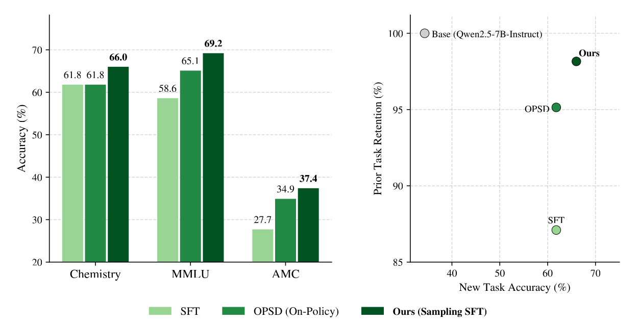
Two measures (§5.1). New task accuracy is accuracy on the task’s test set; for math it also covers AMC, MATH500 and GSM8K as out-of-distribution tests. Prior capabilities is accuracy on benchmarks from other domains: for chemistry and medical these are MMLU, GPQA, AMC, MATH500 and GSM8K, and for math they are chemistry, MMLU and GPQA. “All benchmarks are scored based on single-shot accuracy.” Figure 1 adds prior task retention, “the percent of base model performance the finetuned models are able to maintain”.
What the method is compared with (§5.1).
- SFT on the expert traces as they are, which the paper calls vanilla SFT.
- Rewrite SFT: “a variant of SFT using our sampling proposal prompt to rewrite each expert trajectory; i.e., ‘0th order MCMC’”.
- OPSD, on-policy self-distillation, “which distills from the base model conditioned on privileged information”.
- For math only, “since the rollouts are easily verifiable”, two RL baselines: GRPO, and UFT, “which uses the off-policy expert traces as privileged information during rollout generation”.
Of these, only GRPO learns without the expert traces.
Settings (§5.1). The sampler runs with block size B = 32, a maximum sequence length T = 1856 and 10 MCMC steps. SFT runs are tuned over 1 or 2 epochs (up to 6 for medical), three learning rates and three batch sizes. OPSD uses the hyperparameters of Shenfeld et al. (2026), and the RL baselines the defaults of Liu et al. (2025).
Tools taken from earlier work. The Metropolis-Hastings algorithm (Metropolis et al., 1953; Hastings, 1970). The information projection (Csiszár, 1975). Metropolis-Hastings run block by block on a language model, from the authors’ earlier work on power sampling (Karan and Du, 2025). Putting the expert solution in the prompt to get correct rollouts (Qu et al., 2026; Shenfeld et al., 2026). The baselines: OPSD (Shenfeld et al., 2026; Zhao et al., 2026), GRPO (Shao et al., 2024) and UFT (Liu et al., 2025).
The argument, claim by claim
Claim 1: expert traces can be made on-policy by sampling
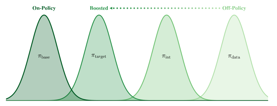
Among the distributions that keep the content of the expert traces, one is closest to the base model. A Metropolis-Hastings sampler started at an expert trace moves toward it, and every step brings the data closer to the base model in KL divergence.
The formal setup is in §4.1. Fix a query. C is the set of trajectories equivalent to its expert trajectory, under “a task-dependent notion of ‘correctness’ or ‘semantic equivalence’”. For math and science that is any trajectory “leveraging information from expert trace x_i that results in a correct final answer”, and for fact learning, one with the same factual content “as judged by an automated (LLM) grader”. P_C is the set of distributions that put all their mass on C (Definition 1). The expert data comes from some distribution in P_C, which may be far from the base model p.
Evidence. First three propositions.
- The target (Proposition 1, §4.1). The information projection of p onto P_C is the member of P_C with the least KL divergence from p. It is “the restriction of the base model onto equivalent trajectories”: p_C(x) is proportional to p(x) for x in C, and zero elsewhere. This is what the sampler aims at, “the closest distribution to the base model that also maintains the information content of the off-policy expert traces”.
- The sampler can stay inside C (Proposition 2, §4.2). Start the chain at the expert trace and use only information-preserving proposals, ones that keep every candidate in C. Then “Running Metropolis-Hastings with irreducible proposals κ and target distribution p_C is equivalent to running MH with information-preserving proposals κ_C and target distribution p.” The constraint moves out of the target and into the proposer, and candidates are scored by the base model’s likelihood alone. Karan’s thread puts it this way: “we switch from using the constraint as a verifier to using it in-context to generate candidates, which are then refined according to base model likelihoods” (post 6).
- Every step moves the data closer (Proposition 3, §4.2). Write π_k for the distribution of candidates after k steps from the expert data. Then the KL divergence from the base model cannot rise from one step to the next, KL(π_(k+1) ∥ p) ≤ KL(π_k ∥ p) for every k, by the data processing inequality. In the paper’s words, the procedure “progressively shifts the original expert policy to informational-equivalent policies that get progressively closer to the base model distribution”.
Then the algorithm as built for a language model (§4.3, Algorithm 1). It works block by block. A prefix is extended by B tokens drawn from the proposal. Then, for each MCMC step, an index is picked at random, everything after it is drawn again from the proposal, and the new candidate is accepted or rejected. The result is fixed as the prefix for the next block. The proposal is the base model itself, prompted with the question, the expert solution and the partial trace, and told: “Starting with the partial response, continue in your own words, including the thinking process.” The authors name the algorithm for its target: “Since our Metropolis-Hastings procedure targets sampling from the information projection given information constraints C, we refer to our sampling algorithm as projection sampling.”
Then three measurements of what the algorithm produced.
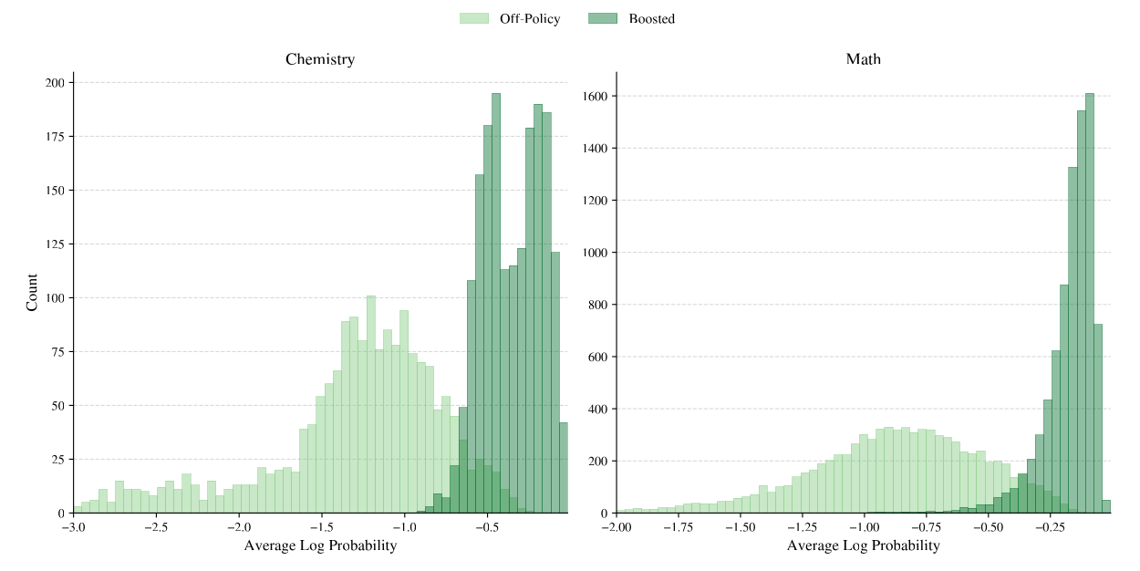
The likelihood of the traces under the base model rises. Histograms of average log-likelihood, before and after, are given for chemistry and math: “The on-policy projection is apparent, yielding traces that are much higher-likelihood relative to the base model while preserving correctness.” (§5.3, Figure 3.)
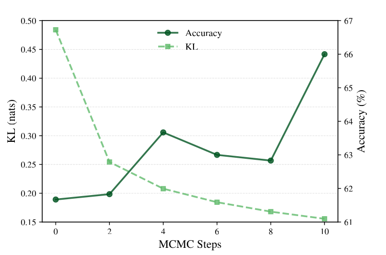
The KL divergence from the base model falls as steps are added. For Qwen2.5-7B-Instruct on chemistry the sampler is run for 0, 2, 4, 6, 8 and 10 steps, where 0 steps is a plain rewrite, and “the boosted data distribution monotonically closes the KL gap with the base model” (§5.3, Figure 5). The text gives no value. The figure’s second line, accuracy after finetuning, belongs to claim 2.
Most of the boosted traces are still correct: 94.33% for chemistry with Qwen and 93.94% with Olmo, 95.33% for math and 95.86% for medical (Appendix C.1).
- Objections it expects.
- That keeping the chain inside C breaks a condition of convergence. “Although this might seem to violate the irreducibility criterion” (§4.2), the acceptance ratio can be rewritten so that a candidate outside C is never accepted, which is Proposition 2.
- That Metropolis-Hastings is too slow on whole sequences. A direct implementation “is infeasible as it requires regenerating full-length token sequences with repeated LLM inference calls” (§4.3). The answer is the block-by-block scheme of Karan and Du (2025), in which sampling each block gives “a strong initialization” for the next.
- That the prompt does not keep candidates in C. “In practice, we find that this prompt can sufficiently generate correct trajectories from expert demonstrations, satisfying the constraint of information-preservation.” (§4.3.) The figures of Appendix C.1 are the measure of it. In his reply to a question about the code, Karan says the assumption is that instruction-following enforces the constraint, “but again, empirically this is inexact”, and that correctness is checked after sampling: “we had post-generation filtering, where rerun on incorrect MCMC traces outside instead of inside the loop, which results in around 95% correctness on average”.
- That the acceptance step is not the one in Algorithm 1. Appendix C.2 says so: the exact rule “can require two forward passes through an LLM per iteration”, so “we approximate the swapping condition by swapping whenever we generate a higher likelihood candidate than the current”. This has “the effect of much more aggressively shifting to high-likelihood regions under the base model”, and the check offered is Figure 5. Karan’s reply calls the rule “a deterministic likelihood-improving acceptance rule”.
- That the sampling is expensive. It is paid once, on the training set: “projection sampling only incurs a one-time cost” (§4.3). Equation 9 estimates it in tokens as the size of the dataset times the number of steps times T squared, over 4B.
- How strongly it is made. The propositions are stated flatly, for the exact sampler. The algorithm is “an approximate sampling algorithm” (§1), and the set C is taken as given: “For theoretical purposes, we assume the existence of such an equivalence relation a priori” (§4.1). Of the implementation as run, Karan’s reply says that “these approximations maintain the effect we care about, which is much more on-policy trajectories with consistency well sustained. In other words, an ‘existence proof’ that an algorithm like this is worth doing.”
- What it hands on. A boosted dataset for each base model and task: “to construct our boosted dataset for finetuning, we simply apply Algorithm 1 to each query-trajectory pair in our expert dataset D” (§4.3). Appendix A prints six traces before and after.
Claim 2: SFT on the boosted data rivals on-policy posttraining, often generalizing better and forgetting less
Plain SFT on the boosted data gains more on the new task than SFT on the expert traces and loses less of what the model could do before. Set against OPSD and RL, the paper’s own summary is that sampling “enables SFT to generalize and retain prior capabilities at least as well as, if not better than, its on-policy posttraining counterparts” (Table 1).
Evidence. The main results are for the Qwen models (§5.2, Table 1). The table below gives, for each task, accuracy on the new task and the average over the prior-capability benchmarks. For math the new-task figure is the table’s average over MATH(3,4,5), AMC, MATH500 and GSM8K. A dash marks a method the table has no row for.
| Method | Chem. new | Chem. prior | Math new | Math prior | Med. new | Med. prior |
|---|---|---|---|---|---|---|
| Base model | 0.343 | 0.597 | 0.318 | 0.422 | 0.353 | 0.597 |
| SFT | 0.618 | 0.520 | 0.242 | 0.389 | 0.448 | 0.353 |
| Rewrite SFT | 0.613 | 0.558 | – | – | 0.457 | 0.512 |
| OPSD | 0.618 | 0.568 | 0.302 | 0.404 | 0.466 | 0.501 |
| GRPO | – | – | 0.457 | 0.414 | – | – |
| UFT | – | – | 0.452 | 0.421 | – | – |
| Sampling SFT | 0.660 | 0.586 | 0.534 | 0.420 | 0.458 | 0.516 |
| Sampling SFT + RL | – | – | 0.567 | 0.430 | – | – |
On chemistry, sampling SFT improves on the base model “by +31.7%, exceeding even the improvement yielded by the on-policy OPSD by +4.20%”, and it “does not lose any MMLU knowledge and reduces the average loss in prior task accuracy down to just -1.10%” (§5.2). Figure 1 shows the chemistry result.
On math, where “vanilla SFT leads to a drop in performance across the board in math benchmarks”, sampling SFT gains +18.0% on MATH(3,4,5), +14.4% on AMC and +20.3% on GSM8K, “on par with the boosts obtained by either RL algorithm”, and +33.7% on MATH500, “surpassing the next best performing (RL) baseline by +26.9%” (§5.2).
On medical, “sampling recovers a 16.3% loss in average prior capabilities with vanilla SFT, and again, forgets the least among all baselines” (§5.2). The text says nothing of medical accuracy on the new task.
Two further results tie the gain to the sampler. Used as the starting point for RL, the sampling SFT checkpoint gives the best math model: GRPO started from it “is the strongest performing model overall, achieving +40.7% performance in MATH500 and +25.1% performance in GSM8K” (§5.2). And as MCMC steps go from 0 to 10 on chemistry, “the corresponding finetuned models trend upwards in accuracy”, which the authors read as “more MCMC steps lead to more on-policy data, which results in better generalization after finetuning” (§5.3, Figure 5, shown under claim 1).
- Objections it expects.
- That one rewrite by the base model would do as well. This is what Rewrite SFT is for: “Simple zero-shot rewrites of the off-policy traces do not perform as strongly in this setting, suggesting the importance of the full MCMC process in Algorithm 1.” (§5.2.)
- That the boosted data is simply better data, for any model. Qwen2.5-7B-Instruct finetuned on chemistry data boosted for Olmo does worse than on the expert traces: “the accuracy on Chemistry drops to 57.33%, which is significantly worse than the other baselines (61.8% for vanilla SFT)” (Appendix B). A 50/50 mix of boosted and original data reaches 62.14%, “in between standard SFT and SFT on the boosted dataset”. The authors’ reading: “The fact that this sampling procedure is custom to the base model distribution is crucial” (§5.2).
- That the gain is paid for in forgetting. “This strong generalization does not come at the cost of catastrophic forgetting.” (§5.2.)
- That this is one model family. Olmo-3-7B-Instruct on chemistry is given “to demonstrate that our method applies to a variety of pretrained model families” (Appendix B). In Table 2 sampling SFT has 0.583 on chemistry and 0.617 on prior capabilities, OPSD 0.597 and 0.600, SFT 0.567 and 0.590, and the base model 0.328 and 0.601.
- How strongly it is made. With hedges of how often, and none of how sure. The sampler “enables SFT to rival prevailing posttraining techniques, often generalizing better” (Abstract); SFT is found “frequently outperforming existing on-policy learning algorithms” (§5); it “can generalize better and forget less than on-policy learning” (Figure 1). The title is stronger, and so is the thread, which opens “SFT is not dead!” (post 1).
- What it hands on. A doubt about what kind of gain this is: “Given that projection sampling pushes off-policy data to be more in-distribution, can our finetuned models still acquire new behaviors beyond just sharpening existing ones?” (§5.3.)
Claim 3: the finetuned model learns more than a sharpening of the base model
Sampling SFT gives the model abilities the base model does not show however many times it is sampled, within the range tested.
Evidence. Pass@k counts a problem as solved “if at least one of k samples is accurate” (Figure 4). It is measured on chemistry for Olmo-3-7B-Instruct: the base model, OPSD and sampling SFT. The paper states what sharpening would look like: “If finetuning with our sampling algorithm was simply sharpening existing capabilities, we would expect our pass@k curve to eventually converge to the base model.” (§5.3.) What it reports instead is “large, consistent gaps in the pass@k rate up to very large k”, and against OPSD, “for k > 2, we see substantial gaps in our pass@k rate relative to OPSD” (§5.3). The text gives no value for the curves.
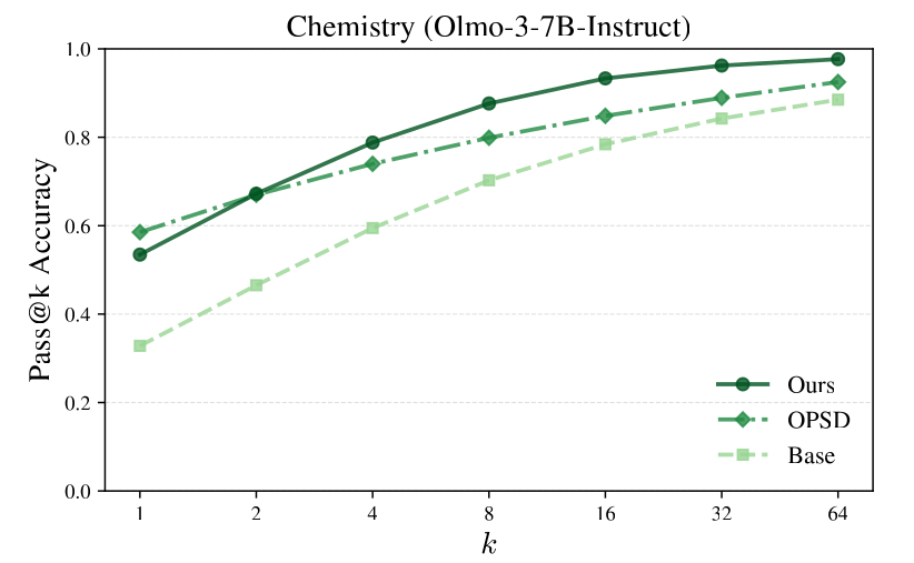
The second piece of evidence is at the level of single problems, ones the base model never solves at the largest k: “some evaluation tasks go from zero pass rate in the base model to pass rates that are up to 67.2% or 53.1%” (§5.3).
- The objection it answers. The claim is itself the answer to an objection, the one claim 2 hands on.
- How strongly it is made. Strongly in the paper. The gaps are “demonstrating that our finetuned model has fundamentally stronger capabilities than the base model” and “indicating that our method enables learning capabilities that OPSD does not learn” (§5.3). The thread is a step softer: “suggesting we are able to introduce genuinely stronger abilities” (post 9).
- What it hands on. The paper’s closing frame, of sampling as “a model-native operator that shapes data for learnability” (§6).
What the paper claims as new
In its own words:
- “rather than modifying the learning objective to accommodate this data, we instead tailor the data distribution to better suit the learner” (Abstract).
- Against earlier ways of joining SFT and RL: “While these approaches alter the learning objective to better account for off-policy data, our approach leaves SFT intact, and instead focuses on modulating off-policy data to be more on-policy.” (§2.)
- Against earlier uses of MCMC with language models: “In contrast, our approach uses sampling to transform off-policy data for subsequent finetuning.” (§2.)
- Three contributions (§1): “a framework that formalizes the task of transforming off-policy data into on-policy data for finetuning”; “projection sampling, an approximate sampling algorithm using Markov chain Monte Carlo (MCMC) techniques”; and results showing that “SFT with sampling can outperform on-policy counterparts like RL and self-distillation on new task generalization as well as prior capability retention”.
- “we introduce a formalism that bridges an apparent disconnect between privileged off-policy information and on-policy training” (§6).
Limits the authors state
The paper has no part given to its limits. These are stated where they come up:
- The equivalence between trajectories that the theory needs is assumed (§4.1).
- Metropolis-Hastings can be slow to converge: “convergence can require exponentially many MCMC steps due to high dimensional sample spaces or poor choice of proposals and initializations” (§4.3).
- The cost grows with the square of the sequence length (equation 9), and the cheaper setting is the less exact one: “We can lower the cost by increasing the block size B, but in general, since projection sampling is a fixed cost, we prefer smaller block sizes that provide higher resolution and less approximation error.” (§4.3.)
- The acceptance step that was run is an approximation of the one in Algorithm 1 (Appendix C.2).
- Not every boosted trace is correct (Appendix C.1).
- RL baselines are run only for math, where “the rollouts are easily verifiable” (§5.1).
- From Karan’s reply: “Admittedly, our implementation for MCMC is expensive as it currently isn’t batched”, and “There is most certainly room for much better practical efficiency”.
How the paper tells it
The paper tells this argument at four lengths: in its title, “Finetuning with Sampling: SFT Learns Better Than You Think”, in the abstract, in the introduction and in the body. This part takes them in that order.
The abstract
Nine sentences. The role is the job the sentence does.
| # | Sentence, abbreviated | Role |
|---|---|---|
| 1 | “Introducing new capabilities to frontier models has long been the goal of posttraining”. | Context |
| 2 | “Conventional wisdom dictates” that RL generalizes and retains, while SFT is “prone to weak generalization and catastrophic forgetting”. | The received view, which the title answers |
| 3 | SFT “can learn from off-policy expert data, whereas RL must rely on a model’s ability to find successful trajectories with repeated sampling”. | What each method lacks |
| 4 | “we seek to leverage the strength of on-policy learning while utilizing the privileged information contained in off-policy data.” | The aim |
| 5 | “rather than modifying the learning objective to accommodate this data, we instead tailor the data distribution to better suit the learner.” | The approach, set against earlier ones |
| 6 | An MCMC sampling algorithm “that progressively transforms off-policy traces to be more on-policy given a reference model for finetuning”. | Claim 1 |
| 7 | Across three kinds of task, the algorithm “enables SFT to rival prevailing posttraining techniques, often generalizing better and forgetting less than strong on-policy baselines”. | Claim 2, with its hedge |
| 8 | The finetuned models “exhibit strong distributional performance and are capable of learning beyond sharpening the base model distribution”. | Claim 3 |
| 9 | Sampling as “a model-native operator that shapes data for learnability”. | Close: the wider use |
The introduction
Nine paragraphs, counting the list of contributions as one. Each with the job it does.
| ¶ | What it says | Role | Cites |
|---|---|---|---|
| 1 | Posttraining has brought “sizeable performance gains across domains like math, science, and coding”. | Context | Guo et al. 2025, Hu et al. 2025, Hendrycks et al. 2021, Li et al. 2022, Rein et al. 2024 |
| 2 | The open question. Evidence “points towards RL as the paradigm of choice”, and SFT forgets. | The problem and the received view | Chen et al. 2025, Chu et al. 2025, Shenfeld et al. 2025, Kirkpatrick et al. 2017, Luo et al. 2023 |
| 3 | The gap is put down to “the on-policy nature of RL”. SFT is off-policy. | The explanation the paper builds on | Chen et al. 2025, Shenfeld et al. 2025, Xiong et al. 2025 |
| 4 | “learning strictly on-policy is also a limitation”: with no correct rollout there is no variance in reward, “resulting in no learning signal”. | What RL lacks | Qu et al. 2026 |
| 5 | For a new capability the model is unlikely to produce a successful trajectory. “Here SFT has an advantage”. | What SFT has | none |
| 6 | Shape the data, and leave the learning algorithm as it is. The question, and a sampling algorithm proposed to answer it. | The question and the approach | none |
| 7 | “Remarkably, this sampling step enables SFT to rival prevailing posttraining techniques”. | The result, in one sentence | none |
| 8 | “Our contributions can be summarized as follows”: a framework, projection sampling, the experiments. | The list of contributions | none |
| 9 | “composing sampling with finetuning is a powerful paradigm”. | Takeaway | none |
The introduction also carries Figure 1, the chemistry result on Qwen2.5-7B-Instruct. Its caption opens with claim 2: “Composed with sampling, SFT can generalize better and forget less than on-policy learning.”
The body, section by section
For each section: its job, how it opens, what it hands on, and what would be missing without it.
§2 Related Works. Its job is to set the claim of novelty against what exists, and it comes before the method. It has three topics under run-in heads. SFT vs. RL takes two paragraphs, one on the gap and its explanations and one on attempts to close it by changing the objective. Self-Distillation ends by naming its baseline, OPSD, “which we refer to as a baseline in this paper”. MCMC Sampling with LLMs covers sampling to a reward, to a program, or to a sharpened distribution. The first and the third end by placing the paper, in the sentences quoted above. Without it, the baselines of §5 arrive unexplained.
§3 Preliminaries. Its job is notation: sequences of tokens, the model as a distribution p over them (equation 1), and the SFT objective (equation 2). Without it, §4 has no p to project.
§4 Boosting Off-Policy Data with MCMC Sampling (claim 1; Figure 2 and Algorithm 1). Its job is the method. It opens with the plan in two steps, a target distribution and then a way to draw from it: “all that remains is for us to explicitly provide an algorithm that samples from it”. A roadmap of its three parts follows.
- §4.1 Targeting the Information Projection. Definitions 1 and 2, and Proposition 1 with its proof. It closes by setting the next part its task: “can we algorithmically evolve samples from q into informational-equivalent but more on-policy samples from p_C?”
- §4.2 The Metropolis-Hastings Algorithm. Opens “We indeed can”. The acceptance rule, the conditions for convergence (Definition 3), then Propositions 2 and 3.
- §4.3 Projection Sampling for LLMs. Opens with why the direct implementation is infeasible. Algorithm 1, the prompt that serves as the proposal, the name, and the cost.
Without §4.1 there is no target. Without §4.2 there is no reason to expect the data to move toward it. Without §4.3 there is nothing to run.
§5 Experiments (claims 2 and 3; Table 1 and Figures 3, 4 and 5). It opens with what it will show: “We now empirically demonstrate that the trajectories generated by our sampling algorithm enable SFT to break its weak characterization”.
- §5.1 Experimental Setup. Tasks, models, evaluation, baselines, and the settings of the sampler and of training, mostly as lists. Table 1 is set in the middle of it.
- §5.2 Main Results. Two run-in heads, Stronger generalization and Retaining prior capabilities. It sends the reader to §5.3 and Appendix B for Olmo.
- §5.3 Analysis. Three run-in heads. Dataset likelihoods (Figure 3) looks at what the sampler produced. Learning beyond sharpening (Figure 4) is claim 3. Scaling sampling compute (Figure 5) goes back to Proposition 3, which “frames sampling as a natural axis for scaling compute”.
Without §5.2 the title has no evidence. Without §5.3 the sampler rests on its proofs alone, and claim 3 is not made.
§6 Conclusion. Two paragraphs. The first restates the three claims in order. The second looks past SFT: for on-policy distillation the sampler “directly induces a teacher distribution”, and for RL it “can simulate on-policy rollouts for RL on hard tasks where the base model is unable to generate signal”.
§7 Acknowledgements. Funding.
The appendices
Each by the job it does. Appendix C has three parts and no text of its own.
| Appendix | Holds | Job |
|---|---|---|
| Appendix A | Six questions, each with the expert trace and the boosted one: two from chemistry, two from math, two from medical | Examples |
| Appendix B | Table 2, Olmo-3-7B-Instruct on chemistry. Two more runs on Qwen: data boosted for the other model, and a 50/50 mix | Checks: a second model family; the data has to fit the model |
| C.1 | The share of boosted traces that are correct, by task and model | Check: content is kept |
| C.2 | The acceptance rule as it was run | Detail of the implementation |
| C.3 | The proposal prompt for chemistry and the grading prompt for medical | Detail to replicate |
The same three claims at every length
Where each claim appears, from the shortest statement of the paper to the longest, then in the lead author’s thread:
| Where | Claim 1 | Claim 2 | Claim 3 |
|---|---|---|---|
| Title | “Finetuning with Sampling” | “SFT Learns Better Than You Think” | |
| Karan’s first post | “we now introduce sampling to the posttraining stack” | “We found a way to make SFT rival current prevailing posttraining methods” | |
| Figure 1, caption | “Composed with sampling, SFT can generalize better and forget less than on-policy learning.” | ||
| Abstract | sentence 6 | sentence 7 | sentence 8 |
| Contributions, §1 | the first and second | the third | |
| Conclusion, §6 | “By carefully boosting the likelihood of off-policy expert data towards the base model’s distribution” | “can generalize better and forget less than both vanilla SFT and strong on-policy baselines” | “able to learn fundamentally new capabilities that are not present in the base model” |
| Section | §4, with its measurements in §5.3 | §5.2 | §5.3 |
| Main-text figures and tables | Figures 2, 3 and 5 | Figure 1, Table 1 | Figure 4 |
| Karan’s thread | posts 4–7 | posts 1 and 8 | post 9 |
The images on the thread are Figure 2 (post 4), the target written as an equation (post 5), Figure 3 (post 7), Figure 1 (post 8) and Figure 4 (post 9). Post 11 adds something the PDF does not say: “We’ll also be presenting this at NeurIPS!”
Threads
- Aayush Karan answers a question about the code for "Finetuning with Sampling" Alex Nichol posts that the paper's released code does not match the paper. The lead author replies that the code swaps the Metropolis-Hastings acceptance step for a rule that accepts any candidate of higher likelihood, and checks correctness after sampling instead of inside it; he gives the cost that led to each choice, points to the KL curve of Figure 5 as the check, and calls the result an existence proof.
- Aayush Karan on "Finetuning with Sampling" The lead author walks through the paper in twelve posts: the open question of adding capabilities without forgetting, what on-policy learning has and what expert data has, the target distribution and the Metropolis-Hastings sampler that moves expert data toward it, the rise in the data's likelihood, the comparison with RL and OPSD, the pass@k result, and sampling as a tool for the rest of posttraining.
BibTeX
@misc{karan2026,
  title = {{Finetuning with Sampling: SFT Learns Better Than You Think}},
  author = {Aayush Karan and Sitan Chen and Yilun Du},
  year = {2026},
  howpublished = {arXiv},
  eprint = {2610.02140},
  archivePrefix = {arXiv},
  url = {https://aakaran.github.io/finetuning_with_sampling/}
}